
Human Population Genetics and Genomics ISSN 2770-5005
Human Population Genetics and Genomics 2024;4(3):0008 | https://doi.org/10.47248/hpgg2404030008
Original Research Open Access
The Quantitative Genetics of Human Disease: 2 Polygenic Risk Scores
David J. Cutler
1,2

 ,
Kiana Jodeiry
2,3
,
Andrew J. Bass
1,2,†
,
Michael P. Epstein
1,2
,
Kiana Jodeiry
2,3
,
Andrew J. Bass
1,2,†
,
Michael P. Epstein
1,2
Correspondence: David J. Cutler
Academic Editor(s): Joshua Akey
Received: Jan 9, 2024 | Accepted: Jul 21, 2024 | Published: Aug 19, 2024
© 2024 by the author(s). This is an Open Access article distributed under the terms of the Creative Commons License Attribution 4.0 International (CC BY 4.0), which permits unrestricted use, distribution, and reproduction in any medium or format, provided the original work is correctly credited.
Cite this article: Cutler D, Jodeiry K, Bass A, Epstein M. The Quantitative Genetics of Human Disease: 2 Polygenic Risk Scores. Hum Popul Genet Genom 2024; 4(3):0008. https://doi.org/10.47248/hpgg2404030008
In this the second of an anticipated four papers, we examine polygenic risk scores from a quantitative genetics perspective. In its most simplistic form, a polygenic risk score (PRS) analysis involves estimating the genetic effects of alleles in one study and then using those estimates to predict phenotype in another sample of individuals. Almost since the first application of these types of analyses it has been noted that PRSs often give unexpected and difficult-to-interpret results, particularly when applying effect-size estimates taken from individuals with ancestry very different than those to whom it is applied (applying PRSs across differing populations). To understand these seemingly perplexing observations, we deconstruct the effects of applying valid statistical estimates taken from one population to another when the two populations have differing allele frequencies at the sites contributing effect, when alleles with effects in one population are absent from the other, and finally when there is differing linkage disequilibrium (LD) patterns in the two populations. It will be shown that many of the seemingly most confusing results in the field are natural consequences of these factors. Given our best current understanding of human demographic history, most of the patterns seen in PRS analysis can be predicted as resulting from systematic differences in allele frequency and LD. Put the other way around, the most challenging and confusing results seen in cross population application of PRSs are likely to be the result of allele frequency and LD differences, not differences in the genetic effects of individual alleles. PRS analysis is an important tool both for understanding the genetic basis of complex phenotypes and, potentially, for identifying individuals at risk of developing disease before such disease manifests. As such it has the potential to be among the most important analysis frameworks in human genetics. Nevertheless, when a PRS is trained in people with one ancestry and then applied to people with another, the PRS’s behavior is often unpredictable, and sometimes is seemingly perverse. PRS distributions are often nearly non-overlapping between individuals with differing ancestry, i.e., odds ratios for unaffected people with one ancestry might be vastly larger than affected individuals from another. The correlation between a PRS and known phenotype might differ substantially, and sometimes the correlation is higher among people with ancestry different than the one used to create the PRS. Naively, one might conclude from these observations that the genetic basis of traits differs substantially among people of differing ancestry, and that the behavior of a PRS is difficult to predict when applied to new study populations. Differing definitions of genetic effect sizes are discussed, and key observations are made. It is shown that when populations differ in allele frequency, a locus affecting phenotype could have equal differences in allelic (additive) effects or equal additive variances, but not both. They cannot have equal additive effects, equal allelic penetrances, or equal odds ratios. PRS is defined, and its moments are derived. The effect of differing allele frequency and LD patterns is described. Perplexing PRS observations are discussed in light of theory and human demographic history. Suggestions for best practices for PRS construction are made. The most confusing results seen in cross population application of PRSs are often the predictable result of allele frequency and LD differences. There is relatively little evidence for systematic differences in the genetic basis of disease in individuals of differing ancestry, other than that which results from environmental, allele frequency, and LD differences.
Keywordsquantitative genetics, human disease, polygenic risk scores, cross-population risk scores
The latest genome-wide association meta-analyses include over one million individuals and have begun to explain a more appreciable portion of disease heritability, improving our knowledge of the genetic factors underlying many adult-onset conditions to the point where polygenic risk profiling provides clinical utility. For example, approximately 80 loci explain 20% of coronary artery disease heritability, 100 loci explain 20% of type 2 diabetes heritability as estimated from the correlation between close relatives, 20 loci explain 30% of Alzheimer’s disease heritability, 150 loci explain 20% of the familial relative risk of breast cancer, and 100 loci explain 33% of the familial relative risk of prostate cancer [1]. Polygenic risk scores (PRSs) broadly attempt to provide a quantitative measure of an individual’s total genetic risk burden of disease over all susceptibility variants identified by genome-wide association studies [2]. PRSs are most commonly calculated within a testing sample as a weighted sum of the number of risk alleles weighted by their measured effect sizes estimated from an independent GWAS training dataset.
The prediction of individual- and group-level disease susceptibility is one of the most promising uses of polygenic risk information for early detection, intervention, and personal health management. For example, current guidelines recommend women initiate biennial screening mammography at 50 years of age [3]. A breast cancer PRS, together with clinical risk factors (e.g., smoking, BMI), identified 16% of the population who could initiate screening at 40 years old as their risk exceeded that of an average 50-year-old as well as 32% of the population that could delay screening at 50 years old since their risk was lower than that of an average 40-year-old [4]. In this prognostic medical genetic context, a PRS developed in a training study is applied to individuals with unknown phenotype (i.e., not yet diagnosed with disease) in a test population, given their known genotypes. Despite these great strides in characterizing the underlying genetic architecture of human diseases and the obvious potential of polygenic risk profiling, the field is riddled with seemingly perplexing observations that have limited the portability of PRSs between populations – and as a result, limited the overall perceived clinical utility of PRSs.
Martin et al. (2017) used published GWAS summary statistics to infer PRSs across populations for several well-studied traits in an effort to quantify the transferability of polygenic risk prediction, identifying clear directional inconsistencies in these inferred scores. When PRSs for height trained in European-biased genetic studies are tested in African or East Asian populations, both the PRS mean and variance appear to be considerably lower in Africans and East Asians [5, 6]. Based on these PRS distributions, African populations are genetically predicted to be shorter than all Europeans and only minimally taller than East Asians with very little diversity in height, which contradicts empirical observations. Similarly, PRSs for schizophrenia trained in European-biased genetic studies have a considerably decreased mean when tested in Africans compared to all other populations [5, 7]. Thus, African populations are predicted to have significantly lower genetic risk for schizophrenia based on these PRS distributions, despite a similar prevalence and significant shared genetic variation tagged by SNPs for schizophrenia across populations [8]. Similarly, PRSs derived from SNPs trained on European populations appear to underestimate the risk of cardiovascular disease in African individuals [9].
On the other hand, when PRSs for type II diabetes and asthma are trained in multi-ethnic cohorts, the PRS mean and variance are both larger in African populations than any other population tested – underestimating risk in Europeans, Asians, and admixed individuals from the Americas [5, 10, 11]. Despite highly significant overlap of common variant risk for inflammatory bowel disease between African and European individuals, Somineni et al. (2021) found differential performance of PRSs as a function of the training population. PRSs trained in African Americans yielded a 7-fold elevation in IBD prevalence in the top percentile of polygenic risk when tested in African Americans (7.4% prevalence) but underestimated risk when tested in Europeans (2.5% prevalence in top percentile), in addition to explaining more than double the variance with African American compared to European summary statistics [12]. PRSs trained in Europeans yielded comparable 3-fold elevations in the top percentile of polygenic risk when tested in Europeans (3.0%) and in African Americans (2.8%), but the proportion of variance explained by the PRS with African American summary statistics was less than half of the variance explained with European summary statistics [12].
More recently, Jeon et al. (2023) evaluated the efficacy of genomic PRS models of acute lymphoblastic leukemia based on discovery GWAS in either non-Latino Whites, Latinos, or multi-ancestry populations. The PRS trained in non-Latino Whites explained a greater proportion of variance when tested in non-Latino Whites compared to when tested in Latinos and significantly less variance than the PRS trained in Latinos and tested in Latinos [13]. The PRS trained on multi-ancestry GWAS data explained equal proportions of variance when tested in non-Latino Whites and in Latinos, which was significantly more than the variance explained by the PRS trained and tested in non-Latino Whites and comparable to the variance explained by the PRS trained and tested in Latinos [13]. Senftleber et al. (2023) conducted GWAS analyses of lipid traits in Greenlanders and found a PRS using variants from only 11 genome-wide significant signals explained 16.3% of the variance in LDL-cholesterol in Greenlanders, whereas 2 million variants are needed to explain up to 22% of the variance in LDL-cholesterol in Europeans [14].
In a follow-up paper, Martin et al. (2019) assessed the decay of polygenic prediction accuracy for quantitative anthropomorphic and blood panel traits when using European-derived summary statistics. Relative to European individuals, genetic prediction accuracy was 1.6-fold lower in Hispanic/Latino Americans, 1.7-fold lower in South Asians, 2.5-fold lower in East Asians, and 4.9-fold lower in Africans on average [15]. Indeed, PRSs for breast cancer constructed using susceptibility loci derived from European-ancestry GWAS had lower discriminatory ability (areas under the receiver operator curves) and inadequate predictive value for breast cancer risk assessment among Hispanic, African American, and African women [16, 17]. A PRS for breast cancer developed in White European populations demonstrated good discrimination but significant overestimation of breast cancer risk in unaffected Ashkenazi Jewish women, reflected in higher mean PRSs in both cases and controls [18]. Such considerable overprediction of breast cancer risk has the potential to lead to harms through the delivery of enhanced preventive measures such as risk-reducing mastectomies, illustrating the danger of misapplying PRSs across populations.
A simple summary of the PRS literature might state that the informativeness of a PRS is inversely proportional to the “genetic distance” between the population used to estimate the genetic effects and the population where those effects are applied [19]. To a population geneticist, the term genetic distance is almost always defined as a function of the variance in allele frequency between populations. Thus, to a population geneticist, this observation reads very much like the informativeness of a PRS is a function of the variance in allele frequency between populations. Consistent with this intuition, Wang et al. (2020) [20] found that linkage disequilibrium and minor allele frequency differences between ancestries can explain between 70-80% of the loss of relative accuracy of European-based PRSs in Africans for traits like body mass index and type II diabetes. It should be noted, though, that the authors were only able to examine allele frequency and LD at common SNPs, rather than data from whole-genome sequencing. When effect sizes are estimated in admixed (African American) individuals accounting for the effects of all variants in a genetic region, the estimated effect size (measured as a β, see below) for virtually all variants and phenotypes examined appeared to be substantially similar, regardless of the genetic ancestry of the variants [21], although confidence intervals were sufficiently broad that some differences in β’s cannot be ruled out.
While many of these observations seem perplexing at first, they are, in fact, relatively easy to understand and predict from basic quantitative genetics theory. To formally understand PRSs, we will begin with a Kempthorne [22] inspired interpretation of genetic effects [23]. In a Kempthorne modeling framework, a genetic effect is not a fixed immutable quantity but is the average contribution of a genetic factor to phenotype, where that average is taken over all other genetic and environmental factors experienced by individuals. This framework makes modeling of PRS analysis straightforward, but an immediate implication is that if allele frequencies or LD differs between populations then most measures of genetic effect must also differ in predictable ways. In fact, it will be shown that there are very few measures of genetic effect that can be the “same” if two populations differ in allele frequency or LD. On the other hand, if one adopts a more Falconer [24] inspired view of a genetic effect (fixed immutable quantities), then differing LD / allele frequencies between populations imply the populations necessarily have differing means and/or variances for the phenotype in question. If the populations are believed to have similar means and variances, and allele frequencies differ, then in a Falconer view, either the effect of a specific gene cannot be the same, or there must also exist “something else” that differs in a way that exactly negates the effects of the allele frequency / LD difference [23]. The notion of the existence of other factors that repeatedly and precisely undo the effects of differing allele frequency and LD is a bit hard to imagine mechanistically, and even if they do exist, modeling such factors will likely lead to a framework fundamentally equivalent to Kempthorne’s in all meaningful ways. Thus, our attempt to understand PRSs starts with a Kempthorne interpretation of genetic effects.
For the next several sections we will present analysis first for a fully quantitative trait, a phenotype which is effectively continuously distributed in the population. After we will show how to apply and adapt the same analysis framework to binary traits, phenotypes with two states, often diseased or not diseased. Fundamentally, all that we do applies equally well to both types of phenotypes but with somewhat different methods of calculation, and we will eventually unify the analyses by transformation of effect sizes to the liability scale for binary traits. Beginning with a quantitative trait, we assume that the trait is fundamentally finite, with finite moments, but we do not necessarily assume that it is normally distributed [23]. When we require this normal assumption, we will explicitly invoke it, and describe why it is needed. Throughout all of this paper we will attempt to follow the notation and framework established in the first paper in this series.
At the heart of a PRS is the application of genetic effect sizes estimated from one study, called here the “training” study, and then used to predict phenotype in another study, called here the “test” study. In order for this procedure to make sense at all, the investigator must be explicitly assuming that the estimated effect in the training study is similar or the same as the effect in individuals in the test study. Thus, to understand PRS we must first examine what sort of genetic effects might reasonably be assumed to be the same. To be specific, begin by considering a single locus in Hardy-Weinberg equilibrium with two alleles A0 and A1 [23]. Let p be the frequency of the A0 allele and q = 1 − p be the frequency of the A1 allele, and assume that we have labeled the alleles such that p ≥ q.
For a continuous trait, there are at least three measures of effect size that might be thought to be the same between studies: the allelic (also called the additive) effects α0 and α1, the difference in allelic effects β = α1 − α0, and the additive variance Va = 2pqβ2 due to the locus [22, 23]. We will show that if two studies have differing allele frequencies, they must have differing α’s, and while they could have the same β or Va, they can not have both simultaneously, i.e., if two populations have differing allele frequency they might have the same β or the same Va, but not both. This will be clear with formal appeal to definition.
Recall that for all phenotypes P we first normalize so that the average phenotype is zero, E[P] = 0. The definition of the additive effect of allele A0 is the conditional expectation of phenotype given that a randomly picked allele A is A0. Thus, α0 = E[P|A = A0] and α1 = E[P|A = A1]. A consequence of the population having a 0 mean phenotype is
Thus, if two populations have differing allele frequency, differing p, they necessarily have differing additive effects of these alleles, unless there is no effect at all, α0 = α1 = 0. To see this explicitly, if two different populations have allele frequencies p and p* with p > p*, say, and corresponding additive effects α0, α1 and
It is a simple matter of definition. It is impossible for two populations with differing allele frequencies to have the same additive effects of both alleles, unless there is no additive effect for either allele, α0 = α1 = 0.
The most natural measure of genetic effect that might be the same between populations is the difference in the additive effects of the alleles, β = α1 − α0. Two populations can have allele frequencies that differ but still have the same difference in allelic effects, β. However, differing allele frequency necessarily implies additive effects themselves differ between populations. If β = β* but p ≠ p* than
using the fact that allele frequencies sum to one. While the difference in additive effects, β, may be the same between populations, the actual additive effects themselves differ by ratios of the allele frequencies.
Another measure of effects that might be the same between populations with differing allele frequency is the additive variance explained by the SNP, Va = 2pqβ2. If two populations have differing allele frequencies with p > p*, then 2pq < 2p* q* because we have oriented alleles so that p ≥ q. If these two populations have the same additive variance due to this locus,
In this we see that if two populations have the same additive variance at a locus, but differing allele frequencies, the population with the larger difference in allele frequencies must have a larger difference in additive effects. Put more intuitively, the additive variance of a locus can be thought of as the product of the allele frequency variance, 2pq, and the variance due the difference in additive effects, β2. If two populations have equal total additive variance, 2pqβ2, the population with the smaller allele frequency variance, 2pq, must have larger variance due to the difference in additive effects, β2. Thus, if additive variance is the same between populations then differing allele frequencies forces the conclusion of differing allelic effects in the populations.
Human disease studies are often most interested in binary phenotypes, diseased or not diseased. For binary traits generally the only reported effect size is an odds ratio, OR (defined below). There are very practical reasons this is the case [23]. However, to use our quantitative genetics tools, we generally [25] model a binary phenotype as resulting from the existence of a threshold t on an unobserved normally distributed phenotype, L, that we usually call “liability” to the disease in question. Here we make a stronger assumption than needed for most continuous trait analysis: we assume liability is normally distributed, parameterized to have mean 0 and variance 1 for computational convenience. Thus, liability is assumed to follow a standard normal density ϕ(x), with standard normal cumulative distribution Φ(x). The overall population prevalence of the disease, ψ, is uniquely determined by the threshold t (Figure 1), and vice versa.

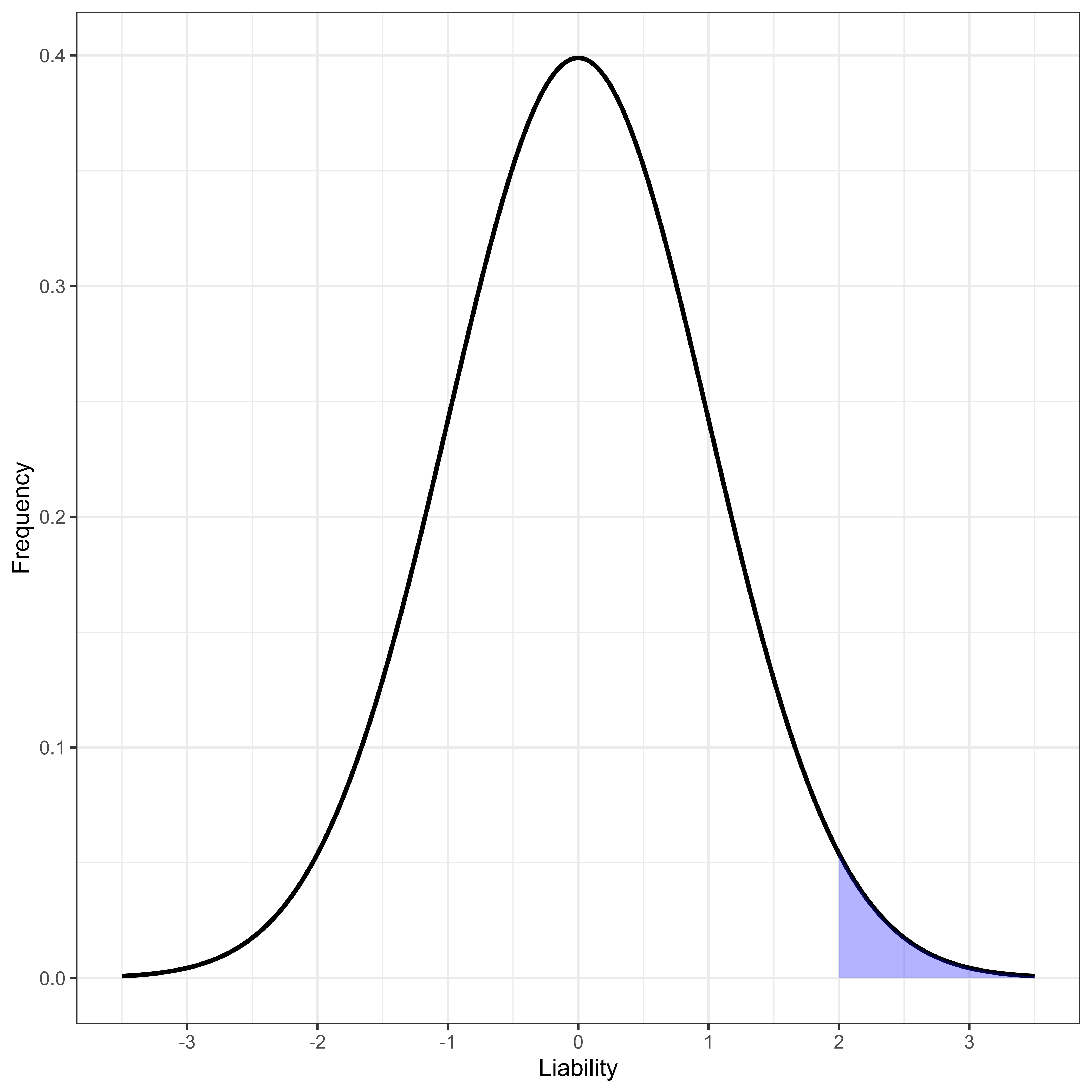
Figure 1 Normally distributed liability with disease-determining threshold at liability greater than 2.
The penetrances, ζ0 and ζ1, of alleles A0 and A1 with additive effects α0 and α1 are defined as the probability an individual is diseased given they have the allele in question. Using the approximation [23] that 1 − Va ≈ 1, as it is for virtually all known alleles contributing to complex disease phenotypes [26],
In this we see that the additive effect of an allele uniquely determines its penetrance, and vice versa. The odds ratio (OR) of allele A1 to A0 is defined as
Presented in this format, it seems far more intuitive that an OR is fundamentally a function of three things: the frequency of the alleles, p, q, the penetrance of alleles, ζ1, and the overall prevalence of the disease, ψ. That it is possible to estimate the OR without explicit knowledge of the prevalence or allele frequency does not change the fact the underlying quantity is per se a function of frequency and prevalence. If two populations have the same odds ratio, OR = OR*, then
Thus, if the odds ratio of allele A1 to A0 is the same in two populations, then the odds of allele A1,
Two populations with same OR can have the same penetrance for an allele if and only if they have the same allele frequency in both populations, p = p*, and the same prevalence in both populations, ψ = ψ*, or the ratio of allele frequencies between the populations is somehow “forced” to be determined in a rather complex way by the penetrance, prevalence and frequency in each population. While we can imagine it is possible for this complex relationship to exist at some particular moment in time, if the allele frequency in either population were to fluctuate slightly, the prevalence and penetrance would have to simultaneously alter in a precise manner to track the allele frequency perturbation. Effectively this can only be true for a disease model where allele frequency, allele penetrance, and population prevalence are all tightly linked together, effectively a Mendelian disorder where the frequency of a variant determines its penetrance and population prevalence. For any complex human disease with many genetic and environmental factors each contributing only a tiny fraction of the total variance, the precise relationship required between the two populations’ allele frequencies, disease frequencies and allelic penetrances will never hold. Put more intuitively, the model where the OR can be the same between two populations naturally arises out of a model where the frequency of a disease is determined by the frequency of the allele. For a complex human disorder where no allele has any strong effect on disease, the frequency of disease is more realistically thought of as nearly independent of the frequency of any one allele, and as such it is impossible for the OR of a complex trait to be the same between two populations with differing allele frequency.
Thus, we arrive at a basic truth. If two populations have differing allele frequency, a locus affecting phenotype could have equal differences in allelic effects (equal β’s) or equal additive variance at this locus (equal 2pqβ2), but not both. They cannot have equal additive effects per se (α’s), equal allelic penetrances (ζ’s), or equal odds ratios (OR’s). An important corollary to this is that if two studies have differing allele frequencies for a particular variant, there is no straightforward way to “average” the odds ratios between the two studies. If one were to perform a “meta-analysis” (usually done as an inverse-variance weighted average) on OR’s generated by two studies with differing allele frequencies, even if the underlying β’s are the same in both studies and the OR’s were both estimated without error, the “meta-OR” will differ from the true value for both studies, and in a very real sense be worse than either. This phenomenon will be seen in a slightly different context in the fourth paper in the series when examining sex-specific prevalence differences. Of course, for a quantitative geneticist the natural way to overcome these concerns is by first transforming effects to the liability scale and performing any sort of averaging / meta-analysis on the β values estimated on the liability scale, not on the OR’s themselves.
As a general rule, PRS analysis begins with the estimation of the effect sizes, generally reported as a β for a continuous trait or as an OR for a binary trait, at a large number of SNPs in a large collection of individuals with some phenotype of interest in the training study. After determination in the training study, effect sizes are generally taken to a different study population, the test study.
Assuming the training study estimated effects at a very large collection of genomewide SNPs, generally the first step in forming a PRS is to “thin” the markers. Thinning markers is a very practical approach to the challenges induced by LD. As discussed in some detail in the first in this series, LD, correlation between allelic states at neighboring SNPs, causes departures from additivity between those neighbors. The combined genetic effect of two markers in LD is, as a rule, very different than the sum of their individual effects, and in many circumstances smaller [23]. In the Kempthorne framework, we see that LD often leads to a “negative” interaction between neighbors, and the joint variance explained by two markers is smaller than the sum of their individual variances. From a Falconer viewpoint, one would say the estimated effect at one SNP is inflated by genetic effects of its neighbors. With this world view, one might intuitively think about a given region where there is only one SNP with a “real” effect, but all of its neighbors who themselves have no “real” effect will have inflated estimated effects caused by LD with the one “real” SNP.
As we previously suggested, there are straightforward approaches to model LD and estimate what effect sizes would be in the absence of LD (i.e., the “true” effects with a Falconer view), but most PRS applications take a slightly different tactic. In the most straightforward approach, often imagining that within any small genomic region only a single SNP will have a large LD-independent effect on phenotype, the SNP with the largest effect in the training study is selected first. Next all other SNPs with sufficiently large LD with the picked SNP are eliminated. This process then repeats, picking the remaining SNP with the largest effect size, and then eliminating all others in high LD with it, until all SNPs have either been picked or eliminated. The collection of picked SNPs, the SNPs after thinning, and their estimated effects will be the set of SNPs used to construct the PRS. There can be innumerable subtle variations on the SNP thinning algorithm [27, 28, 29, 30, 31, 32], including the application of some quite sophisticated machine learning algorithms, but the essential logic for all of them will likely be similar: find SNPs thought to have large effects individually or in combination, remove neighbors whose apparent effects appear to be explained by previously chosen variants, repeat. These processes might use explicit estimates of LD in the process or any sort of surrogate involving physical distances or other measures of correlation in allelic state.
Given a set of n SNPs after thinning, code the genotype of individual j at SNP v as Svj where Svj is the count of the A1 alleles at locus v found in individual j. Thus, Svj = 0 when individual j has genotype A0A0 at locus v; Svj = 1 when the genotype is A0A1, and Svj = 2 when the genotype is A1A1. If βv is the estimated difference in allelic effects at locus v, then the PRS for individual j, PRSj, is usually given by
The quantitative geneticist immediately notices that PRSj is NOT the expected phenotype of individual j! Recall that the expected phenotype of individual j is 0, i.e., E[Pj] = 0. On the other hand, the expected PRS value for individual j is
where αv0 is the additive effect of the A0 allele at locus v. Thus, a PRS calculated in this manner has a mean that differs from the population mean by a constant which is twice the sum of the allelic effects of the A0 allele at all SNPs contributing to the PRS. If two populations have differing allele frequencies, the PRSs will necessarily differ in their mean, because the allelic effects, αv0, necessarily differ. Stated even more straightforwardly, the mean of a PRS is twice the sum across all the SNPs of the β’s multiplied by the population minor allele frequency. There is no escaping the intuition that the PRS mean is fundamentally a measure of allele frequencies. If two populations have differing allele frequencies, they must have differing PRS means, if they have equal genetic effects (β’s).
For binary traits, a PRS is generally calculated under an assumption that OR’s multiply between loci, and therefore the log(OR)’s sum across loci. For person j,
where log(ORv) is the natural log of the OR for SNP v, usually estimated in a logistic regression. This value is often reported with the symbol β to emphasize its natural affinity with effect sizes found in a linear regression. If PRSj is itself normally distributed, perhaps because it is the sum of many factors, then using the fact that for any continuous probability distribution f (x) and continuous function g(x),
whenever the variance (Equation 46) is small. Overall, we see that the mean PRS is a function of the minor allele frequencies in the population in which it is applied. If two populations have differing minor allele frequency, then they have differing average PRS. If individual j’s odds ratio is taken as ePRSj, then this value is meaningful within a population, as it is an approximation to the odds ratio of j to an individual with genotype A0A0 at all loci. However, these values are literally impossible to compare between populations because of the difference in PRS means caused by differing allele frequencies.
Finally it should be noted that a reference person with genotype A0A0 at all loci is unlikely to exist if the PRS included many loci. For instance, if the major allele frequency were 0.9 at every locus, and a 100 uncorrelated loci contributed to the PRS, then fewer than one in a billion individuals would be expected to have reference genotype A0A0 at all loci. Thus, Equation 47 is the odds ratio of real people in the study to a reference individual that could exist in theory, but is very unlikely to be observed. Differing allele frequencies between studies result in differing probabilities the reference individual exists. Differing choice of variants to include in a PRS results in differing reference individuals. Both greater minor allele frequency and more variants will decrease the probability a reference individual actually exists. Thus, in two populations with differing allele frequency, the OR calculated in Equation 47 is a comparison between an individual in the given population to a theoretical individual whose likelihood of existing differs between populations. To the classically trained population geneticist, this analysis will be reminiscent of Ewens’ critiques of the interpretation of genetic load [33].
To give the reader an intuitive understanding of what the above mathematics is describing, here we show a very simple-minded “toy” example demonstrating how changing allele frequency alone can dramatically affect a PRS. The situation described is not meant to be realistic, but instead to illustrate what could happen if there were systematic correlation between minor allele frequency and the direction of effect, combined with systematic differences in allele frequency between training and test studies.
Imagine what might be a “typical” successful PRS, one with 100 different SNPs, all unlinked to one another which in total explain five percent, VPRS/VP = 0.05, of the total phenotypic variance in the training study. For numerical simplicity assume that VP = 1 and that the frequency of the common allele is the same at all loci with p = 0.8, all loci contribute equally to the trait, and so that the difference in allelic effects is the same at all loci with β ≈ 0.03953. Notice that in this toy example the minor allele is associated with increasing trait (liabilty) value at all sites, i.e., the sign of β is positive at all sites. If we were to plot the distribution of PRS across individuals in the training study we would see an approximately normal distribution with standard deviation ≈ 0.22 (Figure 2).
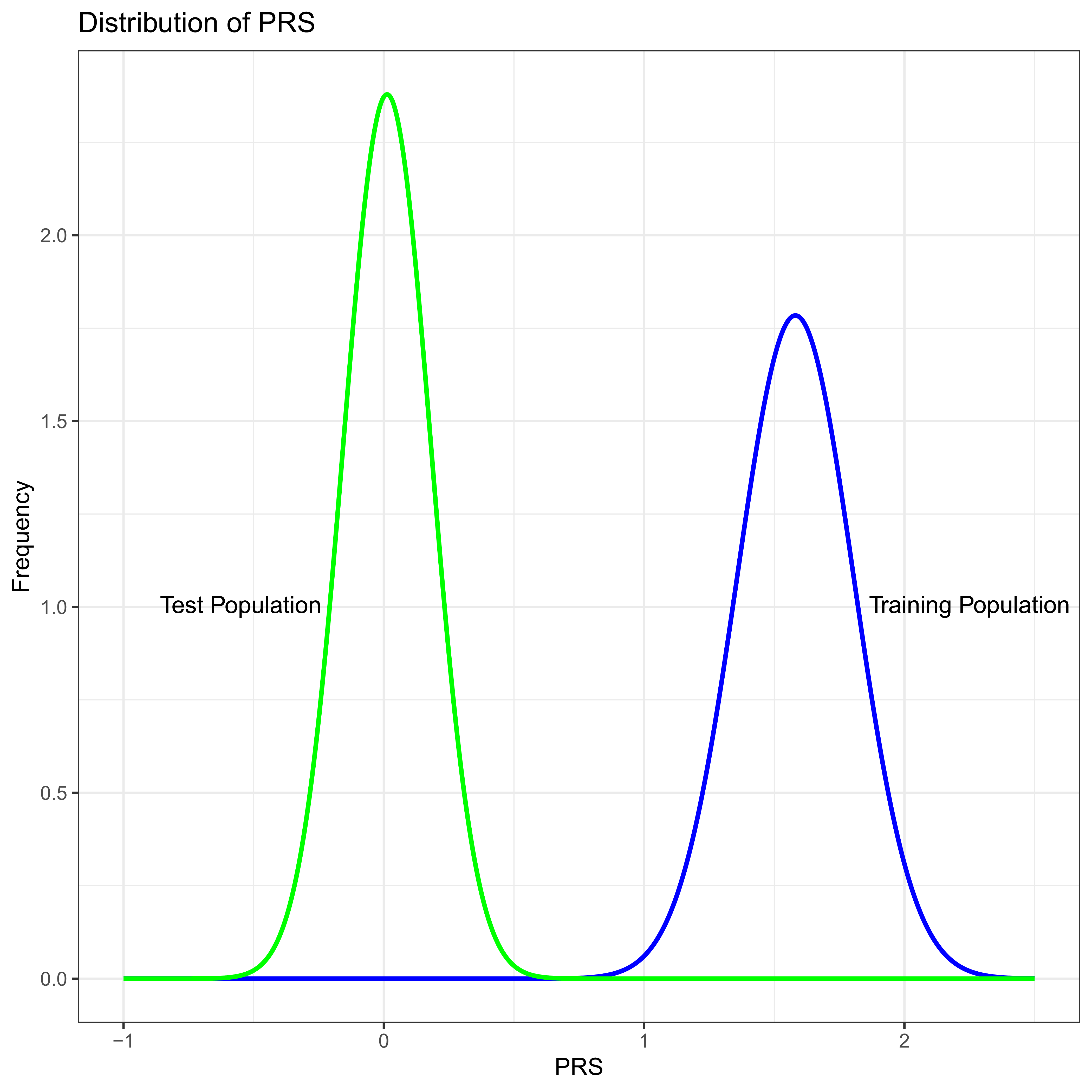
Figure 2 PRS distribution in the training study (Blue) and test study (Green). In this numeric example the only difference between the test and training studies is minor allele frequency which is systematically lower in the test population.
Now suppose we were to apply this PRS in a test study where the difference in allelic effects, β are the same at all 100 SNPs as they are in the training study. However, imagine that by some extremely unfortunate chance all the allele frequencies are different in a systematic way. Imagine that in the second population p = 0.9 at all loci. Thus, in these two populations the genetic effects are exactly the same, and the only difference is in the frequency of the alleles. As is likely to be intuitive to careful readers, the variance due to the PRS, VPRS, in the test population will be less than the training study, because 2pq is smaller at each locus by a factor of
PRSs are seen primarily in two related contexts. In the first context, we might wish to ask to what extent does a PRS developed in one collection of individuals (a training set) accurately predict the known phenotype of individuals in a second study (a test set), where we compare the predicted phenotype to the known phenotype in the test set. In this context we are fundamentally assessing what fraction of the phenotypic variance is explained by the PRS in this new collection of individuals. We could be doing this to compare and contrast differing methodologies used to construct PRSs [28, 34, 35, 36], or we might be doing so to establish the extent to which the phenotype of individuals in the second study appear to have a similar genetic basis as the first [37, 38, 39, 40]. In a different context, we might wish to apply PRSs developed in the training set to predict the unknown phenotype of individuals in the test set, given their known genotypes. It is in this context that a PRS might have significant medical utility [41, 42, 43], if, for instance, individuals with a substantial chance of developing a disease later in life can be identified long before such a condition develops, allowing interventions to be attempted earlier to reduce that risk.
Developers of PRS methodologies frequently wish to show how well PRS predicts phenotype in a test study with known phenotype. For a quantitative phenotype the usual method of evaluation is to calculate the squared correlation between the PRS and the known phenotype, with the notion being increasing squared correlation implies improving PRS. For a perfectly trained PRS, the squared correlation between the PRS and phenotype should converge to the heritability explained by the markers used to construct the PRS whenever there is no dominance within a locus, there are no interactions between genes, nor between genes and the environment, and the state of all genotypes is independent of one another (i.e., no LD between sites contributing to the phenotype). To see this, imagine a PRS where the estimated βv was equal to its true value at all included sites v, and imagine a test study drawn from a population with the same βv at all sites. Letting PRSj and Pj be the PRS and true phenotype of individual j in the test study, and letting SNPs n + 1, …, N be sites contributing to phenotype not included in the PRS, with M environmental factors also contributing, we find
where we use the lack of correlation between genotypes (no LD) extensively, i.e.,
where this adds the assumption of no interaction between any genetic and environmental factors. It should be further pointed out that the allele frequencies and additive effect of the A0 alleles,
Thus, if a PRS in a training study correctly estimates all β’s, and those β’s are shared with the test population, and there are no interactions, the squared correlation between the PRS in the test study and the phenotype of those individuals is the heritability explained by the markers included in the PRS in the test population. The careful reader will have noticed that this proof was made substantially harder looking than it might have been because the PRS does not have 0 mean. Nevertheless, nothing about this changes if the training and test populations have differing allele frequencies, differing additive effects, and therefore differing PRS means, so long as they have the same β’s. Recall though, that we began this section by asserting that the reason one was calculating the squared correlation between PRS and phenotype was as a measure of how “useful” or even “good” a PRS was. We have just shown, though, that this measure is the heritability (additive variance over total variance) of the markers used in the PRS in the test population. We have already seen above that if one population has lower minor allele frequency, the additive variance due to the locus will be less, and therefore heritability due to the marker will be less. So, if a PRS is applied to two different populations, and one of them happens to have lower minor allele frequency at most loci, then the PRS will appear to be “doing worse” in the population with the lower minor allele frequencies, even if all β’s are identical and perfectly estimated. Using the numbers from our toy numerical example, we would find that the correlation between PRS and phenotype was about half (
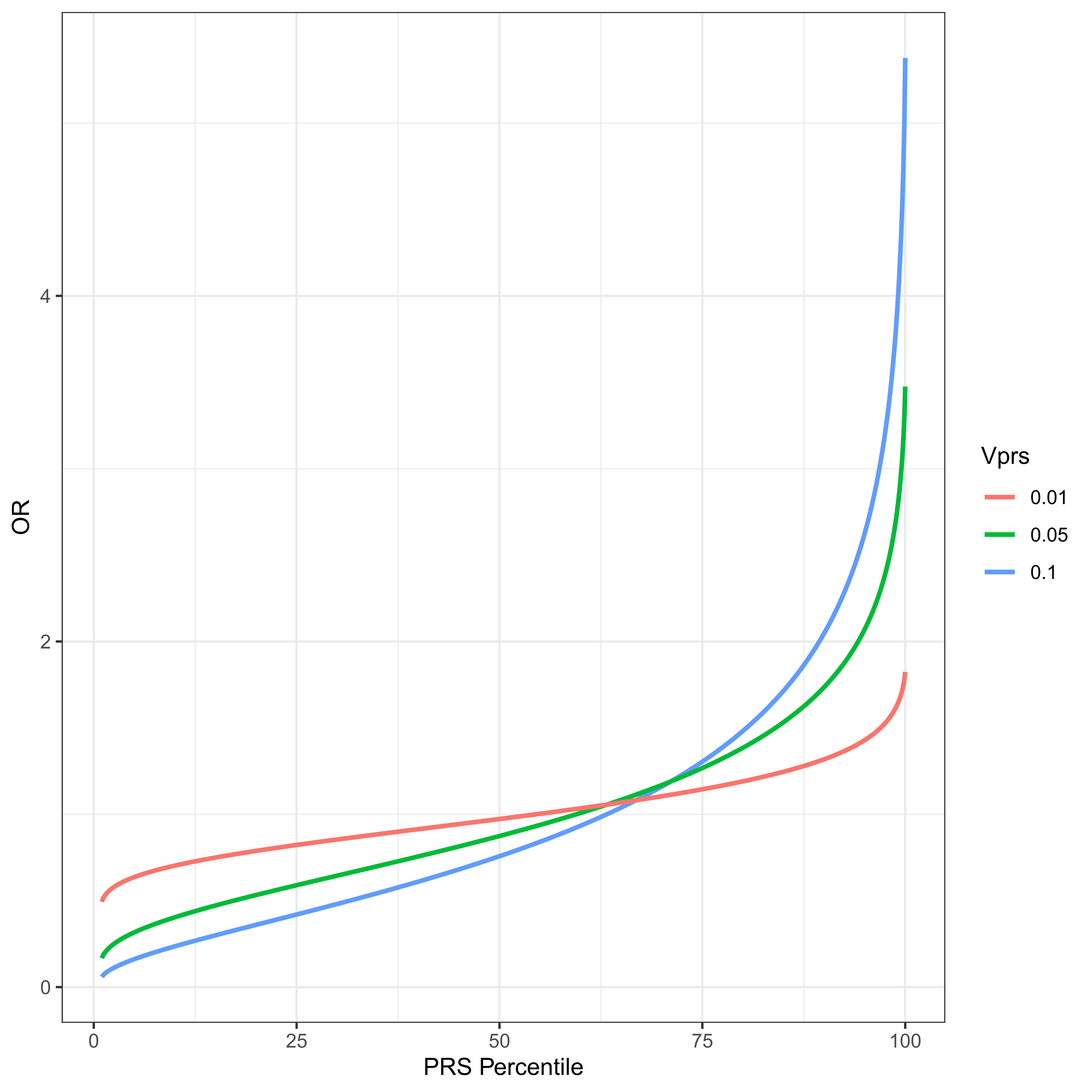
Figure 3 The PRS distribution is divided into percentiles. The odds ratio of average members of a percentile group to average members of the population is plotted for a disease with threshold t = 2, ψ ≈ 0.02275 and VPRS of 1%, 5% and 10% of the total variance. Notice what might appear to be a slightly counterintuitive result. The OR of an individual at the 50th percentile of PRS is necessarily less than 1. This derives from the fact that the residual variance, 1 − VPRS is necessarily less than the total, and an individual at the PRS median has a contribution to phenotype from the PRS loci of exactly 0, the same mean as any randomly chosen individual with unknown PRS. However such a random individual has residual variance 1.
For a binary trait, failure to account for the differences in mean of a PRS between populations with differing allele frequencies can lead to results that appear so mysterious as to be virtually uninterpretable. Recall for a binary trait a PRS is usually calculated with Equation 44 and has mean given by Equation 52. If two test populations have differing minor allele frequencies, the means of their PRS will also differ. For sufficiently large differences in minor allele frequency, the two distributions might not even overlap. Using the values from our toy numerical example (Figure 2), we would discover that virtually no one in the training study had a PRS even remotely close to anyone in the test study, and that their PRS scores are on average ≈ 7 standard deviations apart. If we compared the inferred ORj for individuals between these studies, we would conclude that everyone in one population was vastly more likely to develop disease than anyone in the other population. Recall in this toy example the two populations have identical genetic effects at all loci, but there are systematic differences in allele frequencies.
To simplify the presentation moving forward, we will generally assume that for binary traits OR’s have been converted to effects on the liability scale. After estimating an OR in a training study, we convert the OR to a β value, measured on the liability scale, using prevalence, ψ, and allele frequencies, p and q, from the training study. For any common disorder, a natural approximation would be
For a more rare disorder, where the OR might potentially be very large but ψ small, the simpler approximation of
will likely be more practical. Using one of these estimates for the penetrance of A1, the conversion to effects on the liability scale finishes with
We should remind ourselves that this used the fact that the variance explained by this locus was relatively small. In this fashion, regardless of whether the trait is continuous or binary, we assume the effect sizes have been estimated as a β which represents the difference in allele effects on the phenotype scale for a continuous trait, or on the liability scale for a binary trait. For all that follows whenever we refer to β we mean this value for either a continuous or binary trait, as appropriate. Furthermore, to overcome the problem of PRS means being a function of allele frequency, we will normalize PRS to have mean 0, by using the appropriate allele frequencies, i.e., the allele frequency in the test population when applied to a test population.
One of the most important practical applications of a PRS is to identify individuals at risk of developing a disease who have not yet been diagnosed with such a disease. If a prediction can be made sufficiently early, there is a greater potential for early interventions that may reduce their risk. In this medical genetics application, a PRS developed in a training study is applied to individuals with unknown phenotype in the test population. This is done to identify individuals with unusually large PRSs with the understanding that individuals with unusually large PRSs have unusually high probability of developing disease. Here we find the potential of this approach is determined by the variance explained by the PRS, VPRS, in the test population.
To model this, assume a binary disease with threshold t and total prevalence ψ. Continue to assume that the PRS has been normalized to have mean zero and calculated on the liability scale as described above. Also assume that there are a sufficiently large number of nearly independent loci contributing to the PRS so that the score itself is approximately normally distributed with variance explained by the PRS of VPRS, and therefore with variance due to all other factors 1 − VPRS. Imagine dividing the test population into PRS percentiles. The first percentile includes anyone with PRS less than, tp1, and in general tpi, 1 ≤ i ≤ 99 is given by
where Φ–1 is the inverse of a standard normal distribution, and tpi is in units of
where ϕ is a standard normal density. These results are simple applications of the mean of truncated normals [45]. Calling the penetrance of a randomly chosen individual in the ith percentile ζPRSi,
where ORPRSi is the odds ratio of a randomly chosen individual in the ith percentile relative to a randomly chosen individual in the whole population. Figure 3 plots this odds ratio for varying levels of VPRS for a disease with threshold t = 2, and prevalence ψ ≈ 0.02275, i.e., a relatively common disease. The utility of this approach is very much an increasing function of VPRS in the test population. It should also be clear why PRSs are thought to be so promising for medical genetic applications. For a PRS that explains as little as one percent of the total liability for disease, individuals in the highest percentile have an odds ratio over 1.75. For a PRS explaining 10% of the total variance, a PRS in the top 10% gives an odds ratio above two, and a PRS in the top percentile has an odds ratio above 5, which is similar to some of the highest ever estimated single locus contributors to any complex disorder, e.g. the odds ratio of APOE4 for Alzheimer Disease has been estimated to be ≈ 4.6 [46]. Odds ratios this large could justify early life interventions intended to reduce risk. These VPRS values are from the test population, and are therefore a function of allele frequencies in the test population.
When PRSs are not calculated with a step that normalize the mean to 0, it has been obvious to many that PRSs for binary traits measured as OR’s cannot be meaningfully compared between studies. To find something that could be compared between studies, some investigators [47] measure the difference in PRS means between cases and controls within a study. The difference between case and control means within one test study might be then compared to the difference in case-control means in a second test study. A larger difference between case and control means might be taken as the PRS performing “better.” By now it is perhaps intuitive that the mean difference between case and control PRS is also fundamentally a measure of the variance due to the PRS, and this case-control difference will vary between studies with differing allele frequencies. To understand why this is, continue to assume that PRS has been converted from the OR scale to the liability scale and normalized to have zero mean, as described above. Furthermore, continue to assume a sufficiently large number of nearly independent loci contribute so that the PRS distribution in the test population is well approximated by a normal distribution with variance VPRS. To find the mean of PRSs in cases (E[PRSj|D]) and controls (
where PRSj is approximately normally distributed with mean 0 and variance VPRS, and the residual liability Rj is also approximately normally distributed with mean 0 and variance VR = 1 − VPRS. Therefore, the mean PRS of diseased individual j with residual liability Rj = x is the expectation of a truncated normal (the PRS distribution) with mean x and variance VPRS. Thus for a disease with prevalence ψ and corresponding threshold t,
To find the difference in average PRS between cases and controls note that
Figure 4 plots the difference between case/control PRS means as a function of VPRS for a disease with threshold t = 2. The difference in mean PRSs between cases and controls is a function of the variance due to the PRS, which is a function of allele frequency. Increasing minor allele frequency increases the variance due to the PRS, and therefore increases the mean difference in the PRS between cases and controls. Populations with differing allele frequencies will therefore have varying differences in PRS mean.
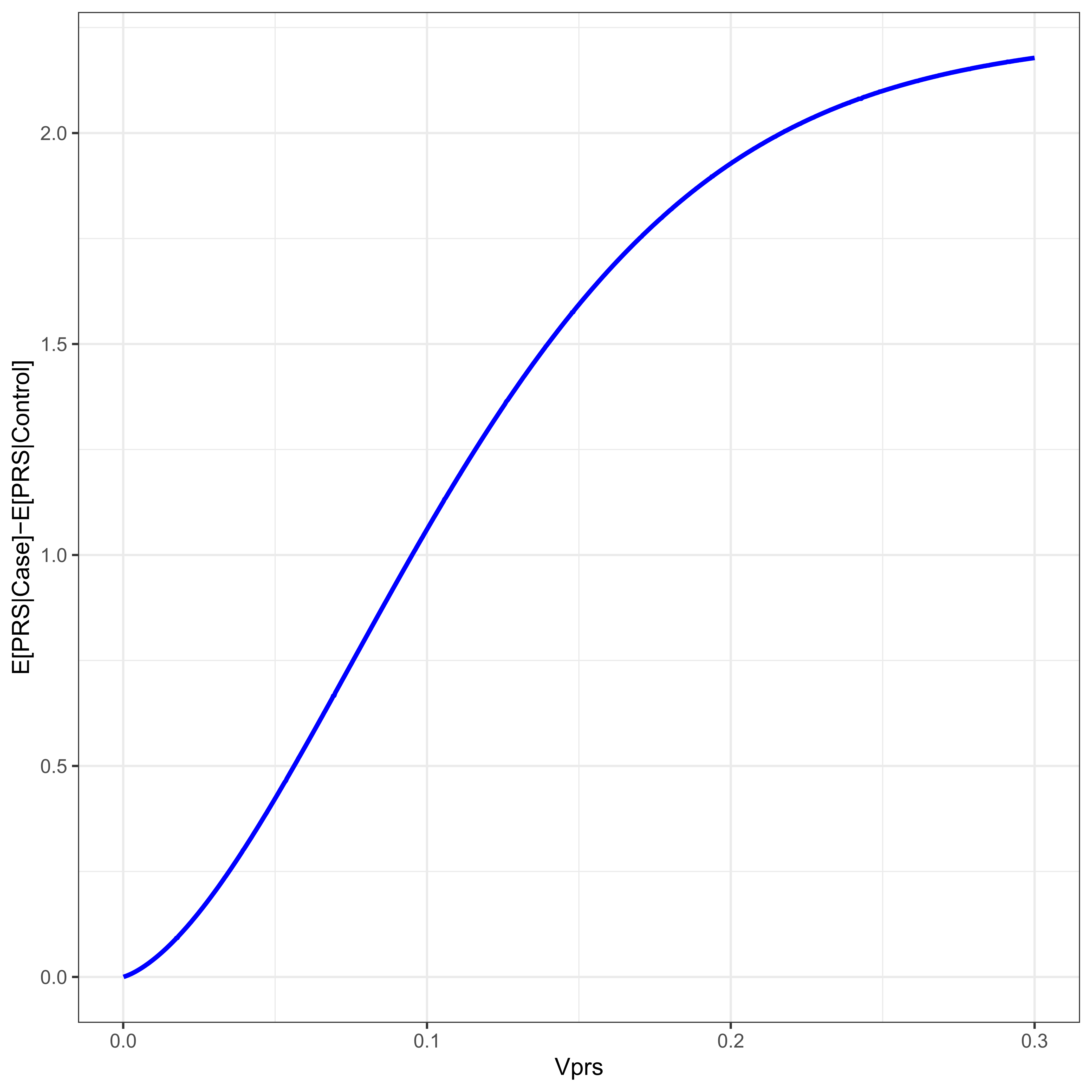
Figure 4 For a disease with threshold 2, ψ ≈ 0.02275, the difference in PRS mean between cases and controls is given as a function of the proportion of the variance due to the PRS, VPRS.
Another approach to evaluating PRS predictive power builds its framework in a machine learning / classification tradition. Here the goal is to find a rule based on the PRS that is used to classify individuals - predict their case/control status from their PRS. In this context the simplest classifier C predicts individual j to be a case if PRSj > C and otherwise predicts j to be a control. For any given value of C we can find the sensitivity, i.e., the “true positive rate” (TPR), the fraction of individuals who are classified as a case and are actually a case, as well as the specificity, i.e., “true negative rate" (TNR), the fraction of individuals j classified as a control who are actually controls.
An arbitrarily large number of classifiers are possible by setting differing values of C, where any given C implies some specific TPR/TNR combination. The overall utility of this classifier is traditionally presented as a receiver operator characteristic curve (ROC), where 1 − TNR, also known as the “false positive rate,” is given on the x axis and the sensitivity on the y. Figure 5 presents the ROC for various value of VPRS found in typical (0.01 ≤ VPRS ≤ 0.1) biobank scale studies of a common complex disease with prevalence a little over 2 percent. Also given is the best possible ROC for that same disease assuming 80% heritability. As is clear, with current study sizes, a classifier based on PRS can achieve a very low false positive rate, almost all individuals classified as cases can be likely cases, by setting a very high threshold on the PRS scale (the top percentile, say), but such a classifier will miss nearly all true cases (poor sensitivity), even for a PRS that explains as much as 10 percent of the total variance. With perfect knowledge of the genetic basis of a trait with 80% heritability, a genetic classifier is still unlikely to be any more useful than a very good “screening tool,” i.e., while it will be possible to identify 95% of individuals likely to develop disease, such a classifier will have a false positive rate of approximately 8%, a value similar to or slightly better than the best prenatal screening tools for Down Syndrome [48].
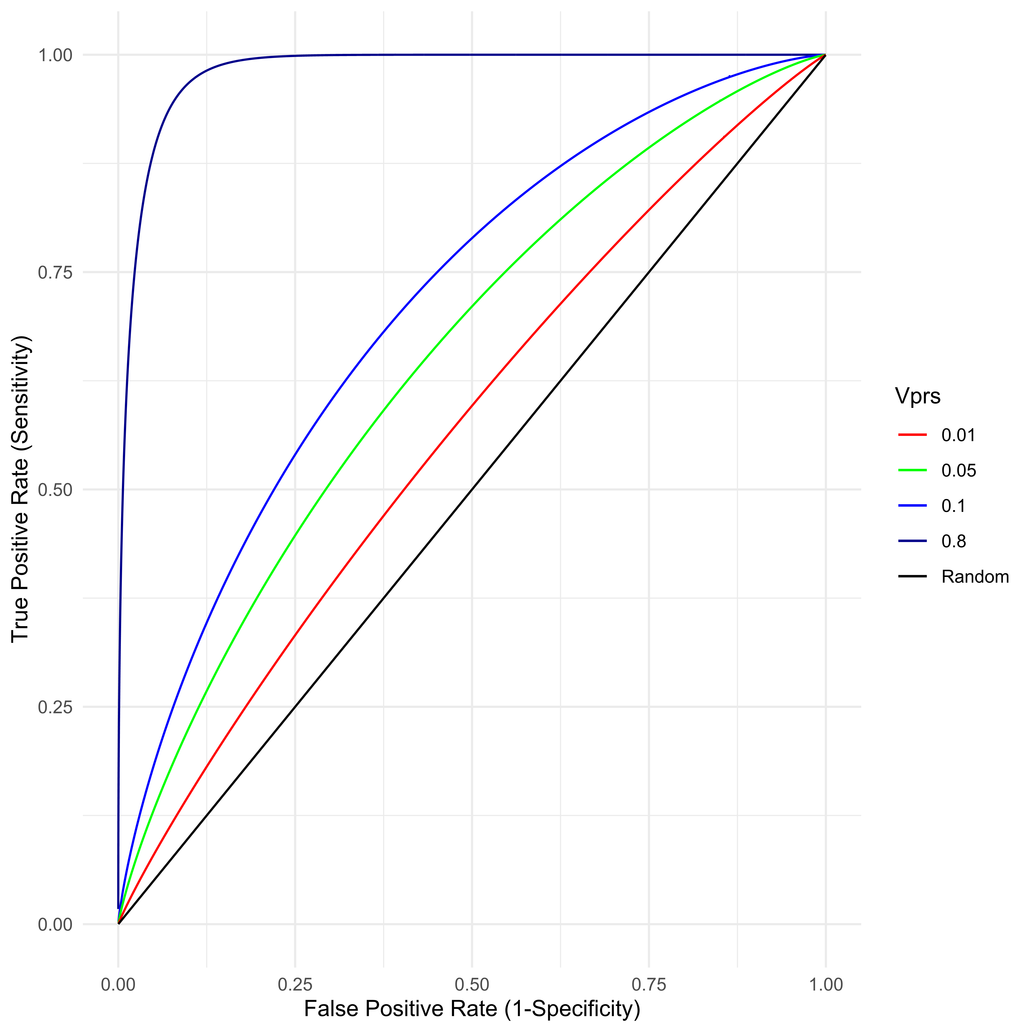
Figure 5 For a disease with true prevalence ψ ≈ 0.02275, the receiver operator characteristic (ROC) is created by classifying samples with a threshold on the PRS. Samples above the PRS threshold are predicted to be cases. Any such classifier’s utility is determined by the VPRS.
It has long been suggested [49] that the field of theoretical population genetics developed largely in the absence of any data sufficient to settle many of the key questions the field wished to understand. Perhaps the most basic question considered by the field is “What is the nature of genetic variation contributing to complex traits?” Theory and analysis surrounding this question reached a highly developed state long before there was anything like sufficient data to test most of the key assumptions introduced by that theory. Now that genetic data and estimates of genetic effects on phenotype are widely available, there is, perhaps less direct appeal to theory developed in the absence of this data than there might be. In this particular case, though, somewhat obscure theoretical results can help build our intuition.
In the human genetics community, the start of the GWAS era was accompanied by what was frequently called the “Common Disease, Common Variant Hypothesis” [50, 51]. Advocates and critiques of this hypothesis were, perhaps often unknowingly, echoing debates that had occurred more than a decade earlier in the theoretical quantitative genetics community. Theoretical quantitative geneticists advocating a view most similar to the Common Disease, Common Variant position were sometimes called “neo-Darwinians” [52]. Those arguing an opposing view were sometimes called supporters of the “infinitesimal” model. While the infinitesimal model has its origins with Fisher [53], the first presentation detailing the connections between individual locus population genetics forces (mutation, selection, and drift) with phenotypic level quantitative genetics measures (variance components, heritability etc.) is due to Lande [54]. In Lande’s development of the infinitesimal model, complex traits result from mutation/selection balance under stabilizing selection. The variants that contribute to traits are a combination of alleles of potentially large effect, but with very low frequency, combined with many common alleles with much smaller individual effects. The neo-Darwinians, often spearheaded by Turelli [55], argued that a substantial fraction of genetic variation was likely contributed by high-frequency alleles of large effect, whose frequency was maintained through balancing selection [56]. At the time these debates were most prominent, there was very little direct evidence to support either view. However, the neo-Darwinians developed several interrelated analyses of the infinitesimal model that they believed diminished the likelihood this view was correct. First, the neo-Darwinians used data from experimental breeding studies, in particular mutation accumulation studies, to argue that if the infinitesimal model was correct it requires that the distribution of allelic effects be highly leptokurtic, i.e., that a substantial fraction of the total genetic variance must be contributed by extremely rare alleles of very large effect. A corollary to this analysis showed most traits must be influenced by very many genes, hundreds or thousands generally [56]. The neo-Darwinian school argued that the only alternative to believing in this worldview was to suppose that a substantial fraction of the variation in complex traits was contributed to by common alleles of large effect, maintained by some form of balancing selection.
Over 20 years of GWAS has convinced nearly everyone in the human genetics community that common alleles of individually large effect generally explain little of the variance for most phenotypes studied, be they traits such as height [57], or common disease phenotypes [26]. This is not to say they never exist (e.g. APOE4 discussed above), but that such examples are very rare. The neo-Darwinian prediction that a significant fraction of the variance in most complex traits would be contributed by a few common alleles of very large effect is usually wrong. The natural conclusion, therefore, is that the infinitesimal model is likely largely correct. Nevertheless, if we are to accept this model, the critiques leveled by the neo-Darwinians are no less cogent. If we accept that there are almost no very common alleles of very large effect, then we must believe most complex disease is contributed to by very many loci and that a substantial fraction of the variation is contributed by rare alleles of large effect, likely scattered throughout many loci across the genome.
Placing these intuitions in the modeling context here, we believe that alleles that substantially increase liability for disease will more often than not be the less frequent allele because in this context, as disease per se can be a factor contributing to the stabilizing selection central to the infinitesimal model [54]. In fact, under a wide range of mutational models and effective population sizes, it may be fundamentally impossible to distinguish the effects of stabilizing selection from simple purifying selection on individual alleles [58].
As we have notated our analysis, the theory above suggests that if a locus contributes to liability to disease, we expect the A1 to be associated with increasing disease liability more often than the A0 allele. Thus, the general theory suggests that we expect α1 > 0 more often than we expect α0 > 0. Moreover, the general theory argues that if α1 ≫ 0 then we expect that q ≪ 0.5, i.e., the alleles with very large effects on liability likely have very small allele frequencies. Put most succinctly, for disease alleles of large effect, q is likely to be small and β = α1 − α0 positive. While, this is our general intuition, if the actual SNPs used to construct the PRS were discovered in a typical case-control design this generalized bias in the sign β can be amplified hundreds of fold.
A typical case-control design for the training study might have close to equal numbers of cases and controls, even for a disorder that is uncommon in the general population. If the frequency of cases in the training study is in excess of its population prevalence, then for the same β2 there is greater power to identify a variant when β > 0. The larger the β and the rarer the disorder the greater the bias. This is easily understood from a simple comparison of the power to detect a variant. The power of any study to detect a significant SNP effect will be proportional to the variance explained by the SNP on the phenotype in the study. If the training study is designed by sampling individuals at random from the population independent of their phenotype, the power to associate a variant with phenotype is proportional to 2pqβ2 and therefore symmetric with respect to the sign of β. However, if the design samples a disproportionately large number of cases relative to population prevalence, it has oversampled individuals with positive liability, and therefore oversampled alleles with positive α’s. This oversampling is greater when β is positive. To understand why, recall that
because p > q. Thus, the allelic effect, α1, of the rare allele necessarily differs from the population mean more than the effect of the common allele, α0. When β > 0 is positive, individuals with the rare allele are closer to the threshold than individuals with the common allele would be were β < 0. For the same value of |β|, the penetrance of a rare risk allele is greater than the penetrance would be for common allele with the opposite sign β. As a result the difference in allele frequency between cases and controls will be larger when the rare allele increases the risk of disease. Noting that the power for any case-control study with an equal number of cases and controls is proportional to (Pr[A0|Case]Pr[A1|Control] − Pr[A1|Case]Pr[A0 |Control])2, for a common disease with ψ = 0.05, the power to find a large effect, β2 = 1, rare allele, q < 0.05, is more than 15 fold greater when β = 1 than when β = −1. For a rare disorder, ψ = 0.001, sites with β = 1 are over 125 times more likely to be discovered than sites with β = −1. This bias to discover positive β sites is true regardless of the magnitude of β, but for sites with modest effect, |β| = 0.1, the power differential is less than a factor of 2 for both common (1.3) and rare disorders (1.7).
Thus, the Neo-Darwinian criticism of the infinitesimal model argues that many of the alleles contributing to any phenotype will have large |β|, and small q, and there is likely to be a bias towards positive β whenever disease itself is a selective factor affecting allele frequency. Regardless of the general bias, a case-control design for a training study will be 10’s or even 100’s of times better powered to discover sites of large effect when β is positive. Even weak β’s should be slightly more commonly discovered in case-control studies when β is positive. There is relatively strong empirical evidence suggesting discovered β’s are generally positive [59, 60]. However, evaluation of empirical evidence is complicated by LD in a manner discussed in some detail below. Nonetheless, we have arrived at the first intuition encapsulated in the toy example. On average we expect there to be correlation between the sign of β and allele frequencies. In the toy example all variants had the exact same sign, which is why we refer to this as a toy example. In real data the correlation will be more subtle, but over many variants and most diseases we expect there to be a meaningful correlation between β and q, with larger positive β associated with smaller q. We expect this bias to be particularly pronounced when the training study samples cases more frequently than population prevalence.
For over 100 years population geneticists have conceptualized a population as a self-contained entity, where one generation promulgates the next via binomial sampling of alleles, a process they generally call Fisher-Wright sampling. Population geneticists generally call alleles “neutral” when their probability of being sampled is independent of their identity and call the change in allele frequency from one generation to the next “genetic drift.” Importantly, the expected frequency of any neutral allele after sampling is the same as its frequency before sampling. Under drift alone, the frequency of a neutral allele is a martingale; a random variable whose expectation the next time it is observed is exactly equal to its current value.
Since the earliest days of fly genetics it was noticed that when a population of flies were kept in a large flask, and then a small number of flies were chosen at random, often by collecting whichever flies happened to move from one flask to the other via the flasks’ “bottleneck,” the frequency of alleles among flies that traveled through the bottleneck were often different. In general, alleles present in the first flask, the “source” bottle, are frequently absent from the second flask, the “destination” bottle. On the other hand, alleles that had been rare in the source bottle are, sometimes, seen in the destination bottle at frequencies much higher than in the source. This phenomenon has long been noted in human disease studies where the fact that many rare, high penetrance, disease alleles were discovered precisely because they were at unusually high frequency in a relatively isolated population [61, 62, 63].
A pair of extant populations may have historically had a source and destination relationship. When this relationship exists we will refer to the extant population which had been the source as the “historical-source” population, and other as the “historical-destination” population. Perhaps counterintuitively, the reason disease alleles are often at unusually high frequency in historical-destination populations is because allele frequency is a martingale unless acted on by strong natural selection. When a destination population was created, the expected frequency of all alleles in the destination population was same as their frequency in the source. However, if the destination population was created by sampling only a relatively small number of individuals from the source population, there is a substantial probability that any rare allele in the source population might not have been sampled and therefore been absent from the destination population, i.e., during a founding event, alleles are lost and are at frequency zero in the destination population. If we think Nf individuals are sampled from the source population to create the destination population then, for an allele A1 with frequency q in the source population, the probability, ω, that A1 is entirely absent from the destination population at the time of founding is the probability that its frequency, q′, in the destination population is zero.
The two in front of Nf derives from diploidy. Obviously, the smaller the number of individuals creating the destination population, Nf, the greater the chance an allele is lost. Similarly, the smaller the initial frequency, q, of an allele, the greater the chance it is lost. For any sufficiently rare allele and small bottleneck size, there will be a substantial probability the allele is lost because of the bottleneck.
Nevertheless, allele frequencies are a martingale. Therefore, E[q′] = q. In the destination population, either the A1 allele will have been lost, in which case its frequency became 0, or it will have been present, in which case its frequency was greater than 0. From the law of total conditional expectation
Therefore alleles that are not lost during the population founding event will have higher average frequency in the destination population than they had in the source population. The rarer the allele and the smaller the number of founders, the greater their frequency will increase, on average, conditional on the allele making it through the bottleneck. Heuristically, we can think of this as a lottery for rare alleles. During the founding event, many rare alleles are losers and will be lost. However, if an allele happens to win, then its allele frequency will likely be higher than it was before.
Thus, at the moment of founding the expected frequency of rare alleles present in the destination population is higher than their frequency was in the source. After this moment of founding, the expected frequency of the alleles in both populations remains a martingale. Thus, at any time after the founding, the expected frequency of an allele present in both populations is higher in the historical-destination population than the historical-source. Of course, the actual frequency in both historical-source and historical-destination populations will drift over time. Nevertheless the average frequency remains higher in the historical-destination population.
That alleles are often at usually high frequency “by chance” in small isolated populations, historical-destinations, has been understood for nearly a century, and generally referred to as a “founder effect” in human genetics. While this phenomenon is widely known, it is, we believe, largely thought of as an isolated “random” effect. That belief starts with the true statement “whenever a bottleneck happens, allele frequencies change, and it is random whether or not the frequency increases or decreases," but fails to recognize that conditional on the allele being present in the historical-destination population, it is more likely to have increased in frequency during the bottleneck than it is to have decreased. Thus, conditional on an allele being observable in the historical-destination population, there is a systematic directionality to its frequency that originated during the founding; bottlenecks increase the frequency (on average) of alleles that survive the event, and this expected frequency in the current historical-destination is whatever it was during the founding. While this analysis contemplates a single founding event, the general logic and framework holds for any subsequent migration between the populations. A rare allele found in only one population before migration will increase in frequency in its new population when it migrates from the larger population to the smaller, and decrease in frequency migrating from the smaller to larger population.
This analysis is precisely correct for neutral alleles and approximates a transient analysis for selected alleles. If we imagine the frequency of the rarer disease allele is being tightly regulated by natural selection in the source population, perhaps because it is under very strong selection and therefore in mutation-selection balance (very large s [64]), then this difference in allele frequency caused by the founding will be present immediately after the bottleneck, but will presumably diminish over time from the effects of selection. In the presence of selection, allele frequency is not a martingale, and no matter how the frequency changed in the destination population, over time sufficiently strong selection will determine the allele frequency in the historical-destination population likely making it more similar to the historical-source if selection acts similarly in both. Under strong selection, the difference in allele frequency between historical-source and historical-destination populations will be on average larger the shorter the time since founding. On the other hand, if selection is weaker, allele frequency will fundamentally be a function of Ns (selection and population size) and the effect of selection on allele frequency will be “relaxed” in the smaller population (but see [65, 58] showing that under many circumstance the dependence on N is often minor). Thus, for “weakly” selected alleles, as long as the effective population size is smaller in the historical-destination population, allele frequency will likely be higher, on average.
Combining this result with the intuition we developed from the infinitesimal model, particularly when variants are ascertained in a case-control framework, we find that we expect the rarer allele, A1, to increase liability for disease more often than the common allele, A0, does, i.e., we expect β > 0 more often than β < 0. We expect the larger the effect on disease the lower the allele frequency, on average (β and q are inversely proportional). We think that when we compare two populations, allele frequencies may differ. If one of the populations is something akin to the historical-source population of the other, we expect many rare disease alleles present in the historical-source population will be absent from the historical-destination population. However, when the disease alleles are present in the historical-destination population, they will be on average at higher frequency than they are in the historical-source population. The careful reader will recognize that we have now described a mechanistic insight for the second major correlation assumed in our toy numerical example. If one population is closer to the historical-source and the other the historical-destination, we will expect there to be systematic differences in allele frequency between them. In our toy example, the training population is analogous to the historical-destination population and the test population to the historical-source. In real data, it will never be that all the variants are at higher frequency in the historical-destination than the historical-source, but on average they should be higher. Thus, we have reached the intuition behind the two fundamental correlations demonstrated in the toy example: positive correlation in the sign of β across sites, and positive correlation in allele frequency across loci. While the toy example was intended to be an extreme example of this, we expect the pattern to be general. Allele frequency differences per se ought to contribute to systematic and predictable differences in PRS.
With these intuitions in mind, we can now predict what we expect to happen when we train a PRS in individuals from one population but test it in individuals from another. We expect allele frequencies to vary between populations. Thus, even if the allele effect sizes measured as β are the same between populations, the differing allele frequencies will cause each locus to contribute slightly different amounts of additive variance to the trait, have slightly different OR’s etc. Absent any other information, we might imagine that the various allele frequency differences across many loci would “cancel” out, and important averages might be approximately the same. However, if one population is the historical-source population, and other population its historical-destination, there will be consistent and predictable effects on PRSs.
Begin by imagining training a PRS in a historical-destination population and testing it in the historical-source population, and assume in both studies no correction was made for allele frequency. Assume that all alleles included in the PRS are truly disease influencing, have their effects accurately estimated as β’s, and all β’s are the same in both the historical-source and historical-destination population. Of course, if an allele is present in both the historical-source and historical-destination population we imagine the reason will often be because the allele was originally in the historical-source population, and was introduced into the historical-destination population at the time of founding, rather than being the result of multiple different mutational events to the same allele, or introduced from one population into the other by migration after the founding event. This assumption is fundamentally equivalent to assuming that the population founding is relatively recent relative to 4Ne generations, where Ne is the effective population size of the historical-source population. For humans with effective population sizes somewhere between 10, 000 and 100, 000 and a generation time of at least 15 years, this is equivalent to assuming the founding events happened less than, say, 150, 000 – 1, 500, 000 years ago, which is a near certainty. Therefore, when an allele is present in both historicalsource and historical-destination populations, we suspect those alleles were present in the historical-source population at the time of the founding event, survived the bottleneck, and will have, on average, higher frequency in the historical-destination population than in the historical-source population. This will not always be true, but we imagine it is true more often than not. In this scenario, on average we expect q in the training study (the historical-destination population) to be on average larger than in the test study. These are the conditions of the toy numerical example. If no correction has been made for allele frequency the PRS will have mean
Because we expect disease alleles to have positive β on average, see Section 2.6, increasing allele frequency q implies an increasing mean PRS. Thus, with no allele frequency correction, we expect the mean PRS to be larger in the training set (historical-destination population) than in the test set (historical-source population). If the disease is being contributed to by sufficiently rare alleles or the bottleneck included sufficiently few people, the means of the PRS could be so far apart that the two PRS distributions do not overlap (our numerical example). Not only will the means of the two PRS distributions differ, but the additive variance accounted for by the PRS will also differ between the two studies,
and we see the variance accounted for by the PRS will be higher in the training (historical-destination) population than in the test (founding, historical-source) population. Recalling that if we measure the effectiveness / utility / goodness of the PRS by the squared correlation between PRS and known phenotype, the training population will have higher squared correlation because it has a larger VPRS. Similarly if we measure effectiveness as something like the difference between case / control PRS means, this too is an increasing function of VPRS. In short, if we train a PRS in a historical-destination population and then test it in the historical-source population we will conclude the PRS “works better” in the training population than it does in the test population even if all genetic effects are identical. Moreover, the means of the PRS distribution will be lower in the test set, with the two PRS distributions potentially showing no overlap. Taken together these two observations could easily lead to the conclusion that the PRS “does not work well” in the test population.
Conversely, if we train the PRS in the historical-source population and test it in the historical-destination population, we might reasonably expect that some of the disease alleles present in the historical-source population will be absent from the test population. The effect of this will be discussed in detail below. However, as a thought experiment let us assume that all disease alleles used for training also happen to be in the test population, perhaps by chance, or perhaps because alleles absent from the test set were not included in the training set due to the fact that the reagent used for genotyping (a genotyping chip, say) in the training population only included SNPs known to be present in many populations. In this circumstance we would see the opposite result. The PRS would appear to have higher mean in the test population than in the training population, and the correlation between PRS and phenotype would be larger in the test population. We might appear to have the paradoxical result that a PRS trained in one population works better in a different population. If the sample sizes were vastly different in the training and test studies, one might be tempted to hypothesize that the PRS working “better” in the test study had something to do with the precision of the β estimates, but here we see the phenomena is entirely consistent with simply training in an historical-source population and testing in a historical-destination one.
We expect many rare alleles present in the historical-source population to be lost in the bottleneck and therefore absent from the historical-destination population. On the other hand, we also expect there to be some recently arisen alleles, post-bottleneck alleles, that are only in one of the two populations because they have only recently come into existence, and there has been insufficient migration between the founding and historical-destination populations post-bottleneck for the allele to be found in both places. Thus, we can think of alleles present in one population but absent from the other as belonging to two classes. The first class are relatively older alleles that existed before the founding and by chance were lost in the historical-destination population. These are alleles that could only contribute to disease in the historical-source population. The second class are relatively younger alleles that have arisen after the bottleneck in only one of the two populations, and could be found in either the founding or historical-destination populations. Assuming the founding event is relatively recent compared to population size, we might reasonably expect the first class to considerably out number the second.
If we train our PRS in the historical-destination population, alleles contributing to disease in the historical-destination population but absent from the historical-source population – class 2 alleles found only in the historical-destination population – will exacerbate the trends described above. These are alleles contributing additive variance in the training set but with q = 0 in the test set. They will decrease the mean PRS in the test set, and decrease the correlation between PRS and phenotype. These alleles make a bad situation worse, if you think of lower correlation between PRS and phenotype as a sign the PRS is worse.
If we train our PRS in the historical-source population, all class 1 alleles and class 2 alleles found only the historical-source population will work to reverse the effects of alleles present in both populations. These alleles have q > 0 in the training population, but q = 0 in the test population, and therefore increase the mean PRS in the training population relative to the test, and contribute to VPRS only in the training population, and therefore increase the correlation between PRS and phenotype only in the training group. Depending on how many of these alleles exist in the training set, we can imagine the mean PRS of the training population being higher, lower, or even approximately equal to the test population. Similarly we can imagine the correlation between PRS and phenotype could be higher, lower, or equal.
Thus, if we train a PRS in a historical-destination population and test it in a the historical-source population we expect the mean of the PRS to be lower in the test population, as will the correlation between PRS and phenotype. On the other hand, if we train in the historical-source population and test in the historical-destination any result is possible. The PRS means and correlation between PRS and phenotype might be higher, lower or equal in the two populations. What is certain, though, is that training in the historical-destination population and testing in the founding (historical-source) population will generally make the differences between the two populations appear to be larger than training in the founding and testing in the historical-destination. This is because class 1 alleles (those lost during the founding event) act in the opposite direction as alleles present in both populations.
Linkage disequilibrium (LD), the non-random association between alleles at different loci, often reinforces this general pattern, but in some circumstances can reverse it. In general, LD between sites causes correlation in effect sizes. Call βv and βw the difference in allelic effects at sites v and w in some real population under study with linkage disequilibrium D ≠ 0 between these sites. Imagine another population, identical in every way to the first, but where sites v and w are not in LD (D = 0), and call
where pv, qv, pw, qw are the allele frequencies at sites v and w. In a Falconer inspired derivation of these results we would call
We note that the equality,
In what is likely a common scenario, consider a situation where SNP w has an effect on phenotype independent of LD, β̃v ≠ 0, but SNP v does not, β̃v = 0. Further assume qv ≥ qw, and site v is included in the construction of a PRS, but site w is not, possibly because site v is included on some widely available genotyping array, and site w is not. In a Falconer construction, we would say site w is the “real” effect site, but site v is an “LD surrogate” included in the PRS. For simplicity assume that there are no other sites in LD with v and w with any LD-independent effects. Thus, if we had included site w in the PRS, and everything were perfectly estimated
The immediate implication is that when D is positive, the sign of βv will be the same as βw. When D is negative the signs flip. If we subscribe to an “infinitesimal” model of complex phenotypes, we expect when |βw| is large, βw will generally be positive and qw small. However, if we include site v in the PRS not w, the sign of βv depends on the sign of D, and the general patterns we describe above hold if and only if haplotypes containing both rare alleles are found more often than expected by chance. Otherwise, βv will more often than not have a negative sign, and all the described relationships reverse. Whether one expects the sign of D to be positive or negative is a complex question involving details of the coalescent tree in this region, and requires a somewhat detailed understanding of population sizes and how they change over time and related features of the demographic ancestry of these individuals. Importantly, when populations differ significantly in LD, the sign of D between the v and w could be opposite, resulting in the sign of βv appearing to flip between populations [66]. There may be no easy rule of thumb here. The situation becomes even more complex when there are multiple sites with effects all of which are in LD with v, but also not included in the PRS. Multiple sites in LD will be explored more broadly in the third paper in this series.
Despite the sign of D being somewhat challenging to estimate as a general rule, several effects of including site v in the PRS rather than site w are immediately clear. First, unless qv = qw and the two sites are in perfect LD, then |βv| < |βw| because
Returning to the question of training a PRS in individuals from one population, but testing in a different population, we find including the “wrong” site to have effects that often accentuate the previously described patterns. On average, a bottleneck has no effects on LD; haplotype frequencies do not change, on average. However, if two sites have significant LD between them in the historical-source population, then necessarily “recombinant” haplotypes (haplotypes created only by recombination between the sites) are far more rare in the historical-source population than either of the minor alleles themselves. Being the most rare haplotype, the chance that recombinant haplotypes are completely lost during the bottleneck is greater than any other haplotype. Thus, for sufficiently small bottleneck sizes, it will not be uncommon for all recombinant haplotypes to be lost during the bottleneck, and LD to increase. Of course, conditional on the recombinant haplotypes surviving the bottleneck, LD will decline, but as a rule of thumb (which we will see in data below), LD will generally be greater in the historical-destination than in the historical-source population.
Larger LD in the historical-destination population implies that |β|’s at site v (the site included in the PRS) will be larger in the historical-destination population, as will the additive variance at site v independent of any allele frequency differences. A PRS trained in the historical-destination population should have a higher mean PRS, and better correlation between PRS and phenotype, from LD alone, reinforcing all the patterns seen from changing allele frequency described above (Section 2.8). A PRS trained in the historical-source population will have lower mean PRS than in the historical-destination and lower correlation between PRS and phenotype due to LD, unless site w is absent from the historical-destination population, in which case the patterns described in Section 2.9 hold. Of course, LD attenuates all this by a factor of
While there is perhaps no complete consensus on the details [67, 68, 69, 70, 71, 72, 73], there is at this point virtually no doubt that the vast majority of human ancestors lived in Africa for much of Hominini history, and in some very real sense all extant populations are ultimately descended from ancient African ones. Without doubt there has been a complex pattern of migration, selection, population loss and re-establishments over human history, but in some real sense all humans trace their ancestry back to Africa. Therefore, in the context we will be considering here, it is not entirely unreasonable to think of studies involving people of recent African ancestry as reflecting the historical-source population, and those with recent ancestry primarily outside Africa as largely reflecting historical-destination populations. Similarly we think of those with recent Finnish or Greenland ancestry as reflecting a historical-destination populations from the broader historical-source European peoples, etc. In all likelihood, individuals identified as Latino may often have a complex ancestry involving relatively recent ancestors from Europe, Africa and the Americas, and thus reflect aspects of both historical-source and historical-destination population history.
The systematic effects of bottlenecks on rare allele frequency is relatively easy to observe. Making the likely assumption that the Finnish (FIN) population [74] was created by a founding event from the non-Finnish European (NFE) population, we would predict that many rare alleles in the NFE sample might be absent from FIN, but conditional on a rare allele being observed in the FIN sample, it will on average be more common than in NFE. Restricting our attention to alleles on chromosome 1 at frequency less than 0.001 overall in humans in gnomADv4 [75] genomes (i.e., allele frequency < 0.001), we observe 21, 332, 691 rare sites found in NFE but not FIN, and thirty times fewer sites, 786, 084 found in FIN but not NFE. On the other hand, of the 967, 157 rare alleles found in both populations, over 70%, 683, 172, are at higher frequency in FIN than in NFE. There results are complicated by the fact that far more NFE samples have been sequenced with high coverage in NFE than in FIN. To account for this, we perform one-sided Fisher’s exact tests on all rare alleles observed in both populations, using the observed sample sizes in NFE and FIN. We perform the tests twice. In one, we test the hypothesis that NFE ≤ FIN. In the other we test the reverse, FIN ≤ NFE. Low p-values (close to 0) indicate that the hypothesis has been rejected, meaning that FIN > NFE, when testing the hypothesis that NFE ≤ FIN.
Figure 6 clearly shows that rare alleles are not at the same frequency in the populations. There are highly statistically significant differences in frequency at many sites, but conditional on the difference being statistically significant at p < 10–6, 98.8% of the time FIN has a higher frequency than NFE (103, 091 vs 1, 226 sites. On the other hand, comparing EAS (East Asian ancestry) to SAS (South Asian ancestry), two groups relatively unlikely to have an historical-source / historical-destination relationship, finds nearly identical numbers of unique rare alleles (4.2 million vs. 4.3 million) and a nearly equal number of variants at higher frequency in each group (2.92 million vs 2.98 million), given they are in observed in both. There are more sites at significantly p < 10–6 higher frequency in EAS than in SAS, but the difference is far less pronounced (65, 978 vs 23, 018 sites). Similarly comparing NFE to the Amish population (AMI) we find nearly 1,000 times more rare alleles in the NFE (over 22 million vs 25 thousand), but given that a rare allele is in both populations, it is at higher frequency in AMI over 95% of the time (92, 547 vs 1, 545). Direct comparisons using gnomAD between NFE and AFR, which is a mixture of African Americans and those of more recent African ancestry, is less straightforward because of the differences in sample size and the often complex ancestry (admixture) of the AFR sample.
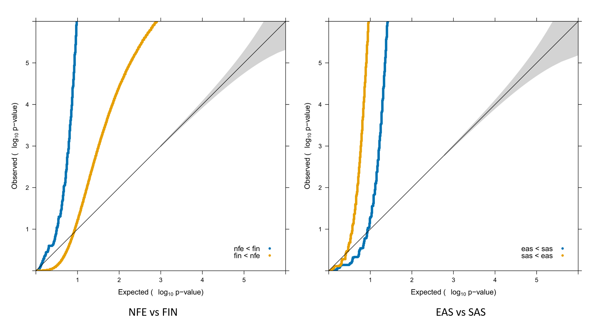
Figure 6 QQ plot testing the equality of minor allele frequency in FIN and NFE for rare SNPs with overall frequency less than 0.001. On the left, in blue and labeled nfe < fin are tests of the hypothesis that the frequency in NFE ≤ FIN. Here a highly significant p-value implies rejection of this hypothesis because the frequency in FIN is greater than NFE. The opposite hypothesis is given in orange, and highly significant results show greater frequency in NFE. There are approximately 100 times as many SNPs at p < 10–6 significantly higher frequency in FIN than in NFE. On the other hand there are only 3 times as many p < 10–6 significantly higher frequency in EAS than in SAS
While we think the effects of bottlenecks will be most pronounced in rare alleles, patterns of LD are usually presented and discussed primarily with reference to common alleles where the effects described above should be much less pronounced. Nevertheless, the expected pattern - LD is less in AFR than in NFE, and NFE tends to show less LD than more recently descended populations - is extremely well established even restricting attention only to relatively common sites [76, 77, 78, 79]. As a simple anecdotal example Figure 7 presents LD [80, 81] patterns for sites with minor allele frequency q > 0.1 (as reported in gnomADv4) in the 150kb surrounding the ESPN locus, a region selected for no better reason than it is on chromosome 1 and shares an abbreviation with a television sports network. In this single example we see that AFR clearly shows less LD than either NFE or FIN and that the differences between NFE and FIN are largely subtle. Patterns of rare allele frequency differences between populations with recent ancestry relationships are, in general, far more pronounced and predictable than LD differences among common alleles.
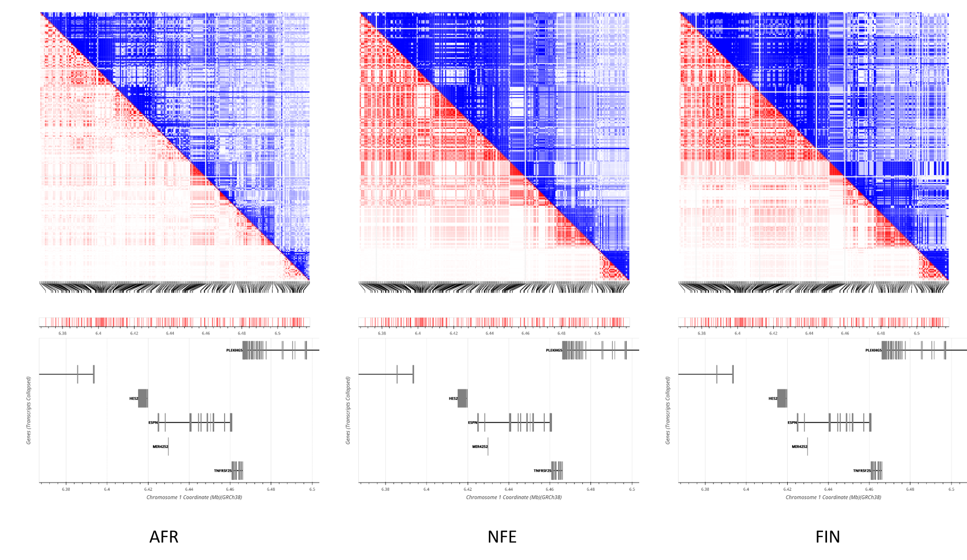
Figure 7 The pairwise LD in the region surrounding ESPN on chromosome 1. Above the diagonal in blue gives D'. Below the diagonal in red shows r2. AFR (left) clearly shows less LD overall than either NFE (center) or FIN (right). NFE and FIN show very similar patterns of LD, with some evidence that FIN may exhibit slightly more LD, particularly as measured by D', but the overall differences are slight, and somewhat inconsistent.
To understand the most challenging observations in PRS analysis, begin by making the following broad-stroke assumptions about human demographic history: African populations are historical-source to all; Latino individuals are a likely mixture of historical-source and historical-destination populations; the broader European population is historical-source relative to Ashkenazi and Greenland populations. In general, rare alleles present in both training and test studies cause training in historical-destination populations and testing in historical-source to have lower PRS mean and variance in the test population than in the training population. Training in the historical-source population and testing in the historical-destination leads to more complex relationships driven by the relative contributions of rare alleles present in both populations versus rare alleles found only in the training population. “Cross-population” training studies (training studies including individuals with diverse ancestries) can benefit from larger sample sizes, but when used with SNP selection methods that are LD aware [82], can also substantially eliminate the complications described in Section 2.10. Cross-population training and SNP selection are also less likely to chose variants for inclusion in the PRS that are absent from some of the training ancestries. Thus, cross-population training is likely to result in better testing performance [83, 44] by picking better SNPs: those whose estimated effects are less influenced by LD and those less likely absent from different populations. Keeping these broad patterns in mind, cross population application of PRS seems predictable and understandable.
When PRSs for height trained in European-biased genetic studies are tested in African samples, both the PRS mean and variance appear to be considerably lower in Africans [5, 6]. Similarly, PRSs for schizophrenia trained in European-biased genetic studies have decreased mean when tested in Africans [5, 7]. PRSs derived from SNPs trained on European populations appear to underestimate (lower PRS mean) the risk of cardiovascular disease in African individuals [9]. Following a similar pattern, a PRS of only 11 SNPs in Greenlanders (historical-destination) had a VPRS = 0.162 for LDL-cholesterol, compared to 2 million variants needed to explain 22% of the variance in LDL-cholesterol in Europeans (source) [14]. PRS models of acute lymphoblastic leukemia [13] trained in non-Latino Whites (historical-destination) explained a greater proportion of variance when tested in non-Latino Whites (historical-destination) compared to when tested in Latinos (mixture of historical-source and historical-destination). Conversely, a PRS for breast cancer trained in the broader European population (source) and tested in Ashkenazi Jewish women (historical-destination) demonstrated good discrimination (an increasing function of VPRS) but significant overestimation of breast cancer risk (higher PRS mean) in the Ashkenazi Jewish [18]. These are all exactly the expected observations when PRS includes a significant contribution from rare alleles present in both populations and at higher average frequency in the historical-destination population.
On the other hand, when PRSs for type II diabetes and asthma are trained in multi-ethnic cohorts (historical-source and historical-destination mixture, but a substantial fraction of historical-destination individuals), the PRS mean and variance are both larger in African populations (historical-source) than any other populations tested (historical-destination) [10, 5, 11]. A PRS for acute lymphoblastic leukemia [13] trained on multi-ancestry GWAS data (historical-source and historical-destination, but historical-destination as the largest contributor) explained equal proportions of variance when tested in non-Latino Whites (historical-destination) and in Latinos (historical-source and historical-destination), which was significantly more than the variance explained by the PRS trained non-Latino Whites (historical-destination, only). Because PRSs trained in historical-source populations can include rare alleles not found in historical-destination populations, we interpret these results as suggesting that both type II diabetes and asthma have significant contributions from rare alleles only found in historical-source populations, as does acute lymphoblastic leukemia, but to a lesser extent.
The observations of Somineni et al. [12] may appear perplexing at first, until one notes that unlike most studies here effect sizes were measured on the liability scale, and PRS mean was adjusted for allele frequency differences. Thus, the differences in PRS between training and test populations were more subtle than generally observed. Nevertheless, a PRS trained in African Americans (source) yielded a higher odds ratio in the top percentile of polygenic risk individuals when tested in African Americans (source) then when tested in Europeans (historical-destination), suggesting the presence of African-specific rare alleles whose effects are most prominent in the PRS tail. On the other hand, a PRS trained in Europeans yielded only slightly higher odds ratios in the PRS tails when tested in European vs African Americans, consistent with the slightly higher VPRS in Europeans likely contributed to by alleles present in both populations but at lower frequency in the historical-source population.
Wang et al. (2020) [20] found that linkage disequilibrium and minor allele frequency differences between ancestries could be used to account for 70-80% of the change in predictive power, a function of VPRS, of PRSs for body mass index and type II diabetes trained in European populations and then tested in both European and African populations. Because this study only included allele frequency and LD measured in common alleles, it is not entirely surprising that there may exist effects of rare alleles not completely accounted for by common allele frequency and LD differences. On the other hand, with whole genome sequencing in admixed individuals [21] using the observed allele frequencies in the tested individuals directly, there was virtually no evidence for any difference by ancestry in effect sizes measured as β’s for any variant (although confidence intervals were often substantial). While the original authors suggest this result might reflect the presence of GxE interactions, the simple minded interpretation is that when the effects of LD and allele frequency can be fully accounted for, genetic effects measured as β’s are the same in all humans. While the examples given here are without question “cherry picked,” as it is nearly impossible not to cherry pick results from a literature with 1000s of examples, it is challenging to find observations that are entirely inconsistent with the patterns described here. We believe that a simple parsimonious explanation of the PRS literature is that β’s are very likely to be generally consistent across human populations. Allele frequency and LD can exhibit complex patterns that may vary considerably by ancestry.
Many of the challenges associated with PRS analysis are largely solved by simply moving to the disease liability scale and being careful to account for allele frequency differences, and consequently differences in PRS mean and variance. For a quantitative disease phenotype (like blood pressure), estimate β at all SNPs in a linear regression, or linear mixed model, in whatever is thought to be a best practice way. For a binary phenotype, estimate the odds ratio in logistic regression or other best practice manner. For the binary phenotype convert the OR’s to penetrances, and then to their allelic effects, α’s, and the difference in allelic effect, β. Thus, we have the “same” measure of effect β on the quantitative phenotype scale for a quantitative disease, or on the liability scale for binary disease. At this stage, one could thin SNPs in a typical way, select sites with large β and remove others in LD with selected sites. Alternatively, one could attempt to use the β estimates and LD regression coefficient matrix to estimate β’s, i.e., the effect size in the absence of LD. This sort of approach is fundamentally similar to [84] and related BLUP (best linear unbiased predictor) estimators of individual variant effect sizes. One would include any SNP with substantial
Nevertheless, if we assume that the estimates are “reliable,” then the SNPs selected and their estimated effect sizes in a training study are available to be applied to any test study, regardless of allele frequency or LD differences, under the simple assumption that
Of course, PRSj is fundamentally an individual measure; it is a property of person j. While we might abstractly think of person j as coming from a particular population, for many people their recent ancestry is likely to be complex, and there is no single value of qv that can be said to reflect their “population.” On the other hand, for any individual with data available from whole genome sequencing, or modern genotyping arrays, there exist several robust methods to infer ancestry [85] that usually report measures that can be viewed as an estimate of the proportion of individual j’s ancestry that comes from given reference populations. Using these estimates as weights combined with reported allele frequencies from gnomAD [75], a “personalized” estimate of qv can be used, qvj, that might be thought of as the allele frequency among individual j’s recent ancestors. In such a manner, with any robust estimates of
Evaluation of a PRS should avoid comparing training to test studies as any reasonable evaluation technique will be a function of VPRS, which is in turn a function of allele frequencies, and potentially personalized ancestry of the individuals, and therefore not directly comparable if the training and test studies include individuals with differing ancestries. Instead the performance of the PRS in the test population should most naturally be compared to its expectations assuming the
For a binary phenotype, the quantity most interesting to the medical geneticist is the probability an individual will ultimately develop disease as a function of their PRS. If Dj is an indicator that individual j will develop disease such that Dj = 1 if the person ultimately develops disease and Dj = 0 otherwise, then
where t is the disease threshold and Φ is a standard normal cumulative distribution. If disease phenotype were known, one could calculate measures such as ROCs for various PRS thresholds etc. Of course, as is obvious from the above, the expectation for these measures is a function of VPRS which is a function of allele frequency and ancestry, and thus not comparable between studies. A natural evaluation technique might be to compare the mean PRS in cases and in controls, or area under the curve (AUC) of the ROC, and ask if the difference in means (AUC) is greater than zero (0.5) - establishing that at least some of the β’s are similar between training and test set, or more quantitatively, if the difference in means (AUC) is consistent with VPRS. Failure to reject equality would argue there is no substantial evidence for a difference in genetic basis of disease in the two studies under comparison.
To understand the effect of these recommendations we use training data from [86] with allele frequency and effect size on Crohns Disease (CD) reported in the GWAS Catalog [87]. The training study consisted primarily of European ancestry individuals (86, 640) meta-analyzed with a much smaller number of East Asian Individuals (9, 846). As the test study we use data from [12] with 1, 335 African Americans with CD and 1, 644 control African Americans. For each individual in the test study, we first estimate the global fraction of their ancestry which derives from each continent using the published gnomAD 4 ancestry PCs [75]. We next calculate a “personalized" allele frequency at each site for each individual in the test study by weighting the gnomAD published allele frequencies for each continental group by the estimated fraction of that individual’s ancestry coming from the continent. Assuming an overall prevalence of CD of 0.00061, we convert reported effect sizes to β’s on the liability scale via Equation 90. We construct the PRS with Equation 130, using the individual’s personalized allele frequency at all sites. The VPRS is calculated using the average over all individuals of the personalized allele frequencies at each site. The associated penetrance of each individual is found via Equation 134, and then converted to an OR relative to a randomly chosen individual. To compare these recommendations to the “standard” methods of presenting PRS, we calculate the a PRS with Equation 44 and the associated OR with Equation 47. First we consider 128 genome-wide significant SNPs identified by the training study authors. All of these SNPs have been identified after fine-mapping and represent the authors’ best estimate of the “casual” variants in each LD region. If these SNPs are directly contributing to phenotype, and the β’s are the same between ancestries, the only difference between training and test studies should be due to allele frequency differences.
Values in Table 1 for the training study use only the reported summary statistics, and should be thought of as akin to their expected values given the reported effect sizes. Values for the test study are the observed values from the test study. Given the allele frequencies at these sites, the VPRS in the test study was estimated as 0.047, very close to the observed values for these individuals, and approximately 10% smaller than the training study. When OR is estimated in the recommended fashion, interpretable results occur. The OR in controls is approximately 1 on average, and 1.3 in cases, suggesting the combined effect of these 128 variants which explain 4% to 5% of the variance have combined to increase the odds of the average case by a factor of 1.3. There is no difficulty in interpreting differences between the training and test study. Using the standard approach leads to values for the PRS and OR that are not immediately interpretable. While the standardly calculated OR in the training study appears slightly different than the OR in test controls, it is likely close enough to avoid any serious interpretation challenges.
Table 1 128 Genomewide Significant SNPs selected after fine-mapping. Means are over individuals studied.

Using more SNPs with less confident estimates of effect size in the training study creates far more difficult interpretation challenges with the standard method. To see this we now select any SNP with a reported p < 10–3 thinning with the simplest possible algorithm. Any selected SNP within a megabase of any other selected SNP is placed in a set. Each set is thinned to a single member by selecting the SNP with the lowest p-value. This rather rudimentary algorithm results in the selection of 574 SNPs (Table 2). Because the p-value threshold is well above multi-test corrected significance, we expect many of the selected SNPs to have no actual effect on phenotype. Their estimated β’s are pure noise. Also, because there was no careful attempt to account for the effects of LD, we expect the selected SNPs to sometimes be in LD with the actual effect sites in complex ways that might differ between studies. Given the personalized allele frequencies, the VPRS was estimated to be 0.119 in the training study, a value certainly inflated by the inclusion of variants not actually contributing to the trait.
Table 2 574 SNPs with p < 10–3. Means are over individuals studied.
Here inclusion of sites with less evidence of effect and poor accounting for LD leads to biased estimates using our recommended procedure. The control mean is clearly larger than 0. It should be slightly less than 0. The observed VPRS in both cases and controls appears biased upward. The estimated OR’s also appear biased upwards. Nevertheless, the effect of including 574 SNPs can be directly compared to using only 128. Using more SNPs increased the difference in PRS and OR means between cases and controls. This strongly suggests that some of the newly included sites contribute to phenotype in a meaningful way. A simple interpretation ensues: some but not all of the newly included sites likely contribute to phenotype, but their effect sizes may be poorly estimated, and LD incompletely accounted for. On the other hand, the standard approach gives values that are exceedingly hard to interpret. The mean PRS in the training study is substantially lower than the control mean from the test study. In fact the difference between the training population and test controls is larger than the difference between test cases and test controls. OR’s show a similar pattern. More pointedly, the OR’s when using 574 SNPs seem to be on a wholly different scale than when using 128 sites. This is presumably because those OR’s are relative to a hypothetical individual with A0A0 genotype at all loci. It is easy to believe that any investigator might find interpretation of the standard PRS values very challenging.
One could further elaborate on this analysis by explicit inclusion of known environmental factors, to either increase the predictive power of a PRS or perhaps to test for a PRS by environment interaction [88, 89]. As discussed in [23], testing for interactions for continuously distributed factors is a complex estimation problem often dependent on the precise distribution of the continuous factors and their scale relative to each other. However, for any combination of discretely distributed factors, testing for interaction is straightforward and not dependent on the phenotypic or factor distribution. Here we illustrate a methodology for discretizing a PRS and combining with a binary environmental variable, but this basic procedure can be extended to any number of categorical environmental variables.
Assume a binary environmental variable E, with two states E0 and E1, with average effect on phenotype P of ϵ0 and ϵ1, respectively for the two states. Estimate the effect of substituting environment E1 for E0, βE = ϵ1 — ϵ0, in a standard way (linear regression or linear mixed model, say), accounting for population structure and other important covariates. For binary phenotypes, estimate the OR of E1 to E0 in a logistic regression / mixed model again accounting for the important covariates, and convert this ORE to βE measured on the liability scale. Thus, for both a continuous or binary phenotype we have the effect measured as βE on the phenotypic / liability scale. If fE0 and fE1 = 1 – fE0 are the frequencies individuals are in state E0 and E1, then the variance due to this environmental factor is
where ej is 0 if individual j has environmental state E0, and 1 otherwise. Of course for a binary phenotype
The simplest method to test for a PRS by environment interaction is to create discrete PRS bins. For sufficiently large sample sizes, one might considered PRS percentile (100) bins as described above. For smaller sample sizes quartile (4) or decile (10) bins might be more appropriate. There are fundamentally two sources of genetic by environment interaction. The first is correlation between genotypic state and environmental state. This can be directly tested in this framework by asking if the frequency of state E1 differs between PRS bins. This test could be asked comparing, perhaps, the first and last bin, or as an “omnibus-test” by asking if the observed variance in the frequency of E1 across bins was greater than expected by chance. If there is significant variation in environmental state between PRS bins, then an interaction exists.
An interaction induced by a correlation between genetic and environmental states is not the only form of interaction that is possible. Regardless of whether or not correlation in state exists between PRS and environment, we say a gene by environment interaction exists if the mean phenotype of an individual with a combination of PRS and environment states differs from the sum of the mean given the environment plus the mean given the PRS. Adapting the notation from [23], and assuming percentile bins, and environmental state Em, m ∈ {0, 1},
where
Polygenic risk scores (PRSs) are a tool of modern human genetics with tremendous potential to help understand the genetic basis of many important human conditions and diseases. Despite its obvious potential, the field is full of perplexing and confusing observations, particularly when applying PRSs developed in one population to individuals from a different population. Here we show that most of these observations can be well understood by a combination of converting binary phenotypes to an unobserved normally distributed liability scale, accounting for allele frequency differences between studies and individuals, and recognizing that many of the measures commonly used to evaluate a PRS are themselves a function of the variance explained by the PRS which in turn is a function of the allele frequencies in the individuals for whom the evaluation is made. PRS analyses themselves provide little evidence that genetic effects differ between populations, other than those induced by differing frequency and LD patterns.
Not applicable.
Not applicable.
Not applicable.
This work is supported by NIH Grants RF1 AG071170 and U01 DK134191.
David J. Cutler is a member of the Editorial Board of the journal Human Population Genetics and Genomics. The author was not involved in the journal’s review of or decisions related to this manuscript. The authors have declared that no other competing interests exist.
All authors participated in the derivation, writing, and editing of this work.
Many of these ideas came from detailed conversations with Patrick Turley, and have been improved and refined by comments from the reviewers and numerous discussions with Greg Gibson.
| 1. | Torkamani A, Wineinger NE, Topol EJ. The personal and clinical utility of polygenic risk scores. Nat Rev Genet. 2018;19(9):581-590. [Google Scholar] [CrossRef] |
| 2. | Chatterjee N, Shi J, García-Closas M. Developing and evaluating polygenic risk prediction models for stratified disease prevention. Nat Rev Genet. 2016;17(7):392-406. [Google Scholar] [CrossRef] |
| 3. | Siu AL, Force UPST. Screening for Breast Cancer: U.S. Preventive Services Task Force Recommendation Statement. Ann Intern Med. 2016;164(4):279. [Google Scholar] [CrossRef] |
| 4. | Maas P, Barrdahl M, Joshi AD, Auer PL, Gaudet MM, Milne RL, et al. Breast Cancer Risk From Modifiable and Nonmodifiable Risk Factors Among White Women in the United States. JAMA Oncol. 2016;2(10):1295. [Google Scholar] [CrossRef] |
| 5. | Martin AR, Gignoux CR, Walters RK, Wojcik GL, Neale BM, Gravel S, et al. Human Demographic History Impacts Genetic Risk Prediction across Diverse Populations. Am J Hum Genet. 2017;100:635-649. [Google Scholar] [CrossRef] |
| 6. | Wood AR, Esko T, Yang J, Vedantam S, Pers TH, Gustafsson S, et al. Defining the role of common variation in the genomic and biological architecture of adult human height. Nat Genet. 2014;46:1173-1186. [Google Scholar] [CrossRef] |
| 7. | Schizophrenia Working Group of the Psychiatric Genomics Consortium. Biological insights from 108 schizophrenia- associated genetic loci. Nature. 2014;511(7510):421-427. [Google Scholar] [CrossRef] |
| 8. | De Candia TR, Lee SH, Yang J, Browning BL, Gejman PV, Levinson DF, et al. Additive Genetic Variation in Schizophrenia Risk Is Shared by Populations of African and European Descent. Am J Hum Genet. 2013;93(3):463-470. [Google Scholar] [CrossRef] |
| 9. | Kim MS, Patel KP, Teng AK, Berens AJ, Lachance J. Genetic disease risks can be misestimated across global populations. Genome Biol. [Google Scholar] [CrossRef] |
| 10. | DIAbetes Genetics Replication And Meta-analysis (DIAGRAM) Consortium, Asian Genetic Epidemiology Network Type 2 Diabetes (AGEN-T2D) Consortium, South Asian Type 2 Diabetes (SAT2D) Consortium, Mexican American Type 2 Diabetes (MAT2D) Consortium, Type 2 Diabetes Genetic Exploration by Next-generation sequencing in multi-Ethnic Samples (T2D-GENES) Consortium, Mahajan A, et al. Genome-wide trans-ancestry meta-analysis provides insight into the genetic architecture of type 2 diabetes susceptibility. Nat Genet. 2014;46:234-244. [Google Scholar] [CrossRef] |
| 11. | Moffatt MF, Gut IG, Demenais F, Strachan DP, Bouzigon E, Heath S, et al. A Large-Scale, Consortium-Based Genomewide Association Study of Asthma. N Engl J Med. 2010;363(13):1211-1221. [Google Scholar] [CrossRef] |
| 12. | Somineni HK, Nagpal S, Venkateswaran S, Cutler DJ, Okou DT, Haritunians T, et al. Whole-genome sequencing of African Americans implicates differential genetic architecture in inflammatory bowel disease. Am J Hum Genet. 2021;108(3):431-445. [Google Scholar] [CrossRef] |
| 13. | Jeon S, Lo YC, Morimoto LM, Metayer C, Ma X, Wiemels JL, et al. Evaluating Genomic Polygenic Risk Scores for Childhood Acute Lymphoblastic Leukemia in Latinos. [Google Scholar] [CrossRef] |
| 14. | Senftleber NK, Andersen MK, Jørsboe E, Stæger FF, Nøhr AK, Garcia-Erill G, et al. GWAS of lipids in Greenlanders finds association signals shared with Europeans and reveals an independent PCSK9 association signal. Eur J Med Genet. 2023;32:215-223. [Google Scholar] [CrossRef] |
| 15. | Martin AR, Kanai M, Kamatani Y, Okada Y, Neale BM, Daly MJ. Clinical use of current polygenic risk scores may exacerbate health disparities. Nat Genet. 2019;51(4):584-591. [Google Scholar] [CrossRef] |
| 16. | Allman R, Dite GS, Hopper JL, Gordon O, Starlard-Davenport A, Chlebowski R, et al. SNPs and breast cancer risk prediction for African American and Hispanic women. Breast Cancer Res Treat. 2015;154(3):583-589. [Google Scholar] [CrossRef] |
| 17. | Wang S, Qian F, Zheng Y, Ogundiran T, Ojengbede O, Zheng W, et al. Genetic variants demonstrating flip-flop phenomenon and breast cancer risk prediction among women of African ancestry. Breast Cancer Res Treat. 2018;168(3):703-712. [Google Scholar] [CrossRef] |
| 18. | Roberts E, Howell S, Evans DG. Polygenic risk scores and breast cancer risk prediction. The Breast. 2023;67:71-77. [Google Scholar] [CrossRef] |
| 19. | Privé F, Aschard H, Carmi S, Folkersen L, Hoggart C, O’Reilly PF, et al. Portability of 245 polygenic scores when derived from the UK Biobank and applied to 9 ancestry groups from the same cohort. Am J Hum Genet. 2022;109(2):373. [Google Scholar] [CrossRef] |
| 20. | Wang Y, Guo J, Ni G, Yang J, Visscher PM, Yengo L. Theoretical and empirical quantification of the accuracy of polygenic scores in ancestry divergent populations. Nat Commun. 2020;11:3865. [Google Scholar] [CrossRef] |
| 21. | Hou K, Ding Y, Xu Z, Wu Y, Bhattacharya A, Mester R, et al. Causal effects on complex traits are similar for common variants across segments of different continental ancestries within admixed individuals. Nat Genet. 2023;55:549-558. [Google Scholar] [CrossRef] |
| 22. | Kempthorne O. The Theoretical Values of Correlations between Relatives in Random Mating Populations. Genetics. 1955;40:153-167. [Google Scholar] [CrossRef] |
| 23. | Cutler DJ, Jodeiry K, Bass AJ, Epstein MP. The Quantitative Genetics of Human Disease: 1 Foundations. Hum Popul Genet Genom. 2023;3:0007. [Google Scholar] [CrossRef] |
| 24. | Falconer DS. Introduction to quantitative genetics. 3rd ed. Burnt Mill Harlow, Essex, England: Longman, Scientific and Technical; 1989. [Google Scholar] |
| 25. | Falconer DS. The inheritance of liability to certain diseases, estimated from the incidence among relatives. Ann Hum Genet. 1965;29(1):51-76. [Google Scholar] [CrossRef] |
| 26. | Loos RJF. 15 years of genome-wide association studies and no signs of slowing down. Nat Commun. 2020;11(1):5900. [Google Scholar] [CrossRef] |
| 27. | Wang Y, Kanai M, Tan T, Kamariza M, Tsuo K, Yuan K, et al. Polygenic prediction across populations is influenced by ancestry, genetic architecture, and methodology. Cell Genom. 2023;3(10):100408. [Google Scholar] [CrossRef] |
| 28. | Kachuri L, Chatterjee N, Hirbo J, Schaid DJ, Martin I, Kullo IJ, et al. Principles and methods for transferring polygenic risk scores across global populations. Nat Rev Genet. 2023;25(1):8-25. [Google Scholar] [CrossRef] |
| 29. | Choi SW, Mak TS-H, O’Reilly PF. Tutorial: a guide to performing polygenic risk score analyses. Nat Protoc. 2020;15(9):2759-2772. [Google Scholar] [CrossRef] |
| 30. | Shi J, Park J.-H, Dua J, Berndt ST, Moy W, Yu K, et al. Winner’s Curse Correction and Variable Thresholding Improve Performance of Polygenic Risk Modeling Based on Genome-Wide Association Study Summary-Level Data. PLoS Genet. 2016;12(12):e1006493. [Google Scholar] [CrossRef] |
| 31. | Speed D, Balding DJ. MultiBLUP: improved SNP-based prediction for complex traits. Genome Res. 2014;24(9):1550-1557. [Google Scholar] [CrossRef] |
| 32. | Zhou X, Carbonetto P, Stephens M. Polygenic modeling with bayesian sparse linear mixed models. PLoS Genet. 2013;9:e1003264. [Google Scholar] [CrossRef] |
| 33. | Ewens WJ. Remarks on the substitutional load. Theor Popul Biol. 1970;1(2):129-139. [Google Scholar] [CrossRef] |
| 34. | Richardson TG, Harrison S, Hemani G, Davey Smith G. An atlas of polygenic risk score associations to highlight putative causal relationships across the human phenome. Elife. 2019;8:e43657. [Google Scholar] [CrossRef] |
| 35. | Fritsche LG, Patil S, Beesley LJ, VandeHaar P, Salvatore M, Ma Y, et al. Cancer PRSweb: An Online Repository with Polygenic Risk Scores for Major Cancer Traits and Their Evaluation in Two Independent Biobanks. Am J Hum Genet. 2020;107(5):815-836. [Google Scholar] [CrossRef] |
| 36. | Wang Y, Tsuo K, Kanai M, Neale BM, Martin AR. Challenges and Opportunities for Developing More Generalizable Polygenic Risk Scores. Annu Rev Biomed Data Sci. 2022;5:293-320. [Google Scholar] [CrossRef] |
| 37. | Power RA, Steinberg S, Bjornsdottir G, Rietveld CA, Abdellaoui A, Nivard MM, et al. Polygenic risk scores for schizophrenia and bipolar disorder predict creativity. Nat Neurosci. 2015;18(7):953-955. [Google Scholar] [CrossRef] |
| 38. | Lobo JJ, McLean SA, Tungate AS, Pea DA, Swor RA, Rathlev NK, et al. Polygenic risk scoring to assess genetic overlap and protective factors influencing posttraumatic stress, depression, and chronic pain after motor vehicle collision trauma. Transl Psychiatry. 2021;11(1):359. [Google Scholar] [CrossRef] |
| 39. | Cleynen I, Engchuan W, Hestand MS, Heung T, Holleman AM, Johnston HR, et al. Genetic contributors to risk of schizophrenia in the presence of a 22q11.2 deletion. Mol Psychiatry. 2021;26(8):4496-4510. [Google Scholar] [CrossRef] |
| 40. | Pillinger T, Osimo EF, de Marvao A, Shah M, Francis C, Huang J, et al. Effect of polygenic risk for schizophrenia on cardiac structure and function: a UK Biobank observational study. Lancet Psychiatry. 2023;10(2):98-107. [Google Scholar] [CrossRef] |
| 41. | Gibson G. On the utilization of polygenic risk scores for therapeutic targeting. PLoS Genet. 2019;15(4):e1008060. [Google Scholar] [CrossRef] |
| 42. | Lewis CM, Vassos E. Polygenic risk scores: from research tools to clinical instruments. Genome Med. 2020;12:44. [Google Scholar] [CrossRef] |
| 43. | Polygenic Risk Score Task Force of the International Common Disease Alliance. Responsible use of polygenic risk scores in the clinic: potential benefits, risks and gaps. Nat Med. 2021;27(11):1876-1884. [Google Scholar] [CrossRef] |
| 44. | Ding Y, Hou K, Xu Z, Pimplaskar A, Petter E, Boulier K, et al. Polygenic scoring accuracy varies across the genetic ancestry continuum. Nature. 2023;618(7966):774-781. [Google Scholar] [CrossRef] |
| 45. | Johnson NL, Kotz S, Balakrishnan N. Continuous univariate distributions. 2nd ed. New York, USA: Wiley; 1995. [Google Scholar] |
| 46. | Tsai MS, Tangalos EG, Petersen RC, Smith GE, Schaid DJ, Kokmen E, et al. Apolipoprotein E: risk factor for Alzheimer disease. Am J Hum Genet. 1994;54(4):643-649. [Google Scholar] |
| 47. | Elliott J, Bodinier B, Bond TA, Chadeau-Hyam M, Evangelou E, Moons KGM, et al. Predictive Accuracy of a Polygenic Risk Score-Enhanced Prediction Model vs a Clinical Risk Score for Coronary Artery Disease. JAMA. 2020;323(7):636-645. [Google Scholar] [CrossRef] |
| 48. | Durković J, Ubavić M, Durković M, Kis T. Prenatal Screening Markers for Down Syndrome: Sensitivity, Specificity, Positive and Negative Expected Value Method. J Med Biochem. 2018;37(1):62-66. [Google Scholar] [CrossRef] |
| 49. | Provine WB. The origins of theoretical population genetics. 2nd ed. Chicago, USA: University of Chicago Press; 2001. [Google Scholar] |
| 50. | Chakravarti A. Population genetics–making sense out of sequence. Nat Genet. 1999;21 Suppl 1:56-60. [Google Scholar] [CrossRef] |
| 51. | Reich DE, Lander ES. On the allelic spectrum of human disease. Trends Genet. 2001;17(9):502-510. [Google Scholar] [CrossRef] |
| 52. | Broadaway KA, Cutler DJ, Duncan R, Moore JL, Ware EB, Jhun MA, et al. A Statistical Approach for Testing Cross-Phenotype Effects of Rare Variants. Am J Hum Genet. 2016;98(3):525-540. [Google Scholar] [CrossRef] |
| 53. | Fisher RA. The Correlation between Relatives on the Supposition of Mendelian Inheritance. Trans R Soc Edinburgh. 1918;52(2):399-433. [Google Scholar] [CrossRef] |
| 54. | Lande R. The maintenance of genetic variability by mutation in a polygenic character with linked loci. Genet Res. 1975;26(3):221-235. [Google Scholar] [CrossRef] |
| 55. | Turelli M. Heritable genetic variation via mutation-selection balance: Lerch’s zeta meets the abdominal bristle. Theor Popul Biol. 1984;25(2):138-193. [Google Scholar] [CrossRef] |
| 56. | Barton NH, Turelli M. Evolutionary quantitative genetics: how little do we know? Annu Rev Genet. 1989;23(1):337-370. [Google Scholar] [CrossRef] |
| 57. | Yengo L, Vedantam S, Marouli E, Sidorenko J, et al. A saturated map of common genetic variants associated with human height. Nature. 2022;610:704-712. [Google Scholar] [CrossRef] |
| 58. | Charlesworth B. Stabilizing selection, purifying selection, and mutational bias in finite populations. Genetics. 2013;194(4):955-971. [Google Scholar] [CrossRef] |
| 59. | Kido T, Sikora-Wohlfeld W, Kawashima M, Kikuchi S, Kamatani N, Patwardhan A, et al. Are minor alleles more likely to be risk alleles? BMC Med Genomics. 2018;11(1):3. [Google Scholar] [CrossRef] |
| 60. | Hernandez RD, Uricchio LH, Hartman K, Ye C, Dahl A, Zaitlen N. Ultrarare variants drive substantial cis heritability of human gene expression. Nat Genet. 2019;51(9):1349-1355. [Google Scholar] [CrossRef] |
| 61. | Knudson AG Jr. Founder effect in Tay-Sachs disease. Am J Hum Genet. 1973;25:108. [Google Scholar] |
| 62. | Levy-Lahad E, Catane R, Eisenberg S, Kaufman B, Hornreich G, Lishinsky E, et al. Founder BRCA1 and BRCA2 mutations in Ashkenazi Jews in Israel: frequency and differential penetrance in ovarian cancer and in breastovarian cancer families. Am J Hum Genet. 1997;60(5):1059-1067. [Google Scholar] |
| 63. | Puffenberger EG. Genetic heritage of the Old Order Mennonites of southeastern Pennsylvania. Am J Med Genet C Semin Med Genet. 2003;121C(1):18-31. [Google Scholar] [CrossRef] |
| 64. | Gillespie JH. Population genetics: a concise guide. 2nd ed. Baltimore, Md, USA: Johns Hopkins University Press; 2004. [Google Scholar] |
| 65. | Gillespie JH. Genetic drift in an infinite population. The pseudohitchhiking model. Genetics. 2000;155(2):909-919. [Google Scholar] [CrossRef] |
| 66. | Wang S, Qian F, Zheng Y, Ogundiran T, Ojengbede O, Zheng W, et al. Genetic variants demon- strating flip-flop phenomenon and breast cancer risk prediction among women of African ancestry. Breast Cancer Res Treat. 2018;168(3):703-712. [Google Scholar] [CrossRef] |
| 67. | Wohns AW, Wong Y, Jeffery B, Akbari A, Mallick S, Pinhasi R, et al. A unified genealogy of modern and ancient genomes. Science. 2022;375(6583):eabi8264. [Google Scholar] [CrossRef] |
| 68. | Wang C-C, Yeh H-Y, Popov AN, Zhang H-Q, Matsumura H, Sirak K, et al. Genomic insights into the formation of human populations in East Asia. Nature. 2021;591:413-419. [Google Scholar] [CrossRef] |
| 69. | Fournier R, Tsangalidou Z, Reich D, Palamara PF. Haplotype-based inference of recent effective population size in modern and ancient DNA samples. Nat Commun. 2023;14(1):7945. [Google Scholar] [CrossRef] |
| 70. | Changmai P, Jaisamut K, Kampuansai J, Kutanan W, Altınışık NE, Flegontova O, et al. Indian genetic heritage in Southeast Asian populations. PLoS Genet. 2022;18(2):e1010036. [Google Scholar] [CrossRef] |
| 71. | Lazaridis I, Alpaslan-Roodenberg S, Acar A, Açıkkol A, Agelarakis A, Aghikyan L, et al. The genetic history of the Southern Arc: A bridge between West Asia and Europe. Science. 2022;377(6609):eabm4247. [Google Scholar] [CrossRef] |
| 72. | Ralph P, Coop G. The geography of recent genetic ancestry across Europe. PLoS Biol. 2013;11(5):e1001555. [Google Scholar] [CrossRef] |
| 73. | Moorjani P, Patterson N, Hirschhorn JN, Keinan A, Hao L, Atzmon G, et al. The history of African gene flow into Southern Europeans, Levantines, and Jews. PLoS Genet. 2011;7(4):e1001373. [Google Scholar] [CrossRef] |
| 74. | Palo JU, Ulmanen I, Lukka M, Ellonen P, Sajantila A. Genetic markers and population history: Finland revisited. Eur J Hum Genet. 2009;17(10):1336-1346. [Google Scholar] [CrossRef] |
| 75. | Wang Q, Pierce-Hoffman E, Cummings BB, Alföldi J, Francioli LC, Gauthier LD, et al. Landscape of multi-nucleotide variants in 125,748 human exomes and 15,708 genomes. Nat Commun. 2020;11:2539. [Google Scholar] [CrossRef] |
| 76. | Lim ET, Würtz P, Havulinna AS, Palta P, Tukiainen T, Rehnström K, et al. Distribution and medical impact of loss-of-function variants in the Finnish founder population. PLoS Genet. 2014;10:e1004494. [Google Scholar] [CrossRef] |
| 77. | 1000 Genomes Project Consortium, Abecasis GR, Altshuler D, Auton A, Brooks LD, Durbin RM, et al. A map of human genome variation from population-scale sequencing. Nature. 2010;467(7319):1061-1073. [Google Scholar] [CrossRef] |
| 78. | International HapMap Consortium. A haplotype map of the human genome. Nature. 2005;437(7063):1299-1320. [Google Scholar] [CrossRef] |
| 79. | Rosenberg NA, Pritchard JK, Weber JL, Cann HM, Kidd KK, Zhivotovsky LA, et al. Genetic structure of human populations. Science. 2002;298(5602):2381-2385. [Google Scholar] [CrossRef] |
| 80. | Lin S-H, Thakur R, Machiela MJ. LDexpress: an online tool for integrating population-specific linkage disequilibrium patterns with tissue-specific expression data. BMC Bioinformatics. 2021;22(1):608. [Google Scholar] [CrossRef] |
| 81. | Machiela MJ, Chanock SJ. LDlink: a web-based application for exploring population-specific haplotype structure and linking correlated alleles of possible functional variants. Bioinformatics. 2015;31(21):3555-3557. [Google Scholar] [CrossRef] |
| 82. | Gao B, Zhou X. MESuSiE enables scalable and powerful multi-ancestry fine-mapping of causal variants in genome-wide association studies. Nat Genet. 2024;56(1):170-179. [Google Scholar] [CrossRef] |
| 83. | Wojcik GL, Graff M, Nishimura KK, Tao R, Haessler J, Gignoux CR, et al. Genetic analyses of diverse populations improves discovery for complex traits. Nature. 2019;570:514-518. [Google Scholar] [CrossRef] |
| 84. | Mathew B, Léon J, Sillanpää MJ. A novel linkage-disequilibrium corrected genomic relationship matrix for SNP-heritability estimation and genomic prediction. Heredity Edinb. 2018;120(4):356-368. [Google Scholar] [CrossRef] |
| 85. | Suarez-Pajes E, Díaz-de Usera A, Marcelino-Rodríguez I, Guillen-Guio B, Flores C. Genetic Ancestry Inference and Its Application for the Genetic Mapping of Human Diseases. Int J Mol Sci. 2021;22(13):6962. [Google Scholar] [CrossRef] |
| 86. | Liu JZ, van Sommeren S, Huang H, Ng SC, Alberts R, Takahashi A, et al. Association analyses identify 38 susceptibility loci for inflammatory bowel disease and highlight shared genetic risk across populations. Nat Genet. 2015;47:979-986. [Google Scholar] [CrossRef] |
| 87. | MacArthur J, Bowler E, Cerezo M, Gil L, Hall P, Hastings E, et al. The new NHGRI-EBI Catalog of published genome-wide association studies GWAS Catalog. Nucleic Acids Res. 2017;45(D1):D896-D901. [Google Scholar] [CrossRef] |
| 88. | Cuesta MJ, Papiol S, Ibañez B, García de Jalón E, Sánchez-Torres AM, Gil-Berrozpe GJ, et al. Effect of polygenic risk score, family load of schizophrenia and exposome risk score, and their interactions, on the long-term outcome of first-episode psychosis. Psychol Med. 2023;53(14):6838-6847. [Google Scholar] [CrossRef] |
| 89. | Nagpal S, Tandon R, Gibson G. Canalization of the Polygenic Risk for Common Diseases and Traits in the UK Biobank Cohort. Mol Biol Evol. 2022;39(4):msac053. [Google Scholar] [CrossRef] |

![]()
Copyright © 2026 Pivot Science Publications Corp. - unless otherwise stated | Terms and Conditions | Privacy Policy


