Investigating population continuity and ghost admixture among ancient genomes

James McKenna; Carolina Bernhardsson; David Waxman; Mattias Jakobsson; Per Sj&#x00F6;din

doi:10.47248/hpgg2404030009

Sections

Abstract
1. Introduction
2. Materials and Methods
3. Results
4. Discussion
Declarations
Appendix
Reference

Human Population Genetics and Genomics 2024;4(3):0009 | https://doi.org/10.47248/hpgg2404030009

Original Research Open Access

Investigating population continuity and ghost admixture among ancient genomes

James McKenna ¹ , Carolina Bernhardsson ¹ , David Waxman ² , Mattias Jakobsson ¹ , Per Sjödin ¹

1. Department of Organismal Biology, Uppsala University, Uppsala, SE-752 36, Sweden
2. Centre for Computational Systems Biology, ISTBI, Fudan University, Shanghai 00433, China

Correspondence: Mattias Jakobsson; Per Sjödin

Academic Editor(s): Daniel Wegmann

Received: Apr 5, 2024 | Accepted: Aug 7, 2024 | Published: Sep 3, 2024

This article belongs to the Special Issue Paleogenomics, ancient DNA, and genomic tales of human history

© 2024 by the author(s). This is an Open Access article distributed under the terms of the Creative Commons License Attribution 4.0 International (CC BY 4.0), which permits unrestricted use, distribution, and reproduction in any medium or format, provided the original work is correctly credited.

Cite this article: McKenna J, Bernhardsson C, Waxman D, Jakobsson M, Sjödin P. Investigating population continuity and ghost admixture among ancient genomes. Hum Popul Genet Genom 2024; 4(3):0009. https://doi.org/10.47248/hpgg2404030009

Abstract

Ancient DNA (aDNA) can prove a valuable resource when investigating the evolutionary relationships between ancient and modern populations. Performing demographic inference using datasets that include aDNA samples however, requires statistical methods that explicitly account for the differences in drift expected among a temporally distributed sample. Such drift due to temporal structure can be challenging to discriminate from admixture from an unsampled, or “ghost”, population, which can give rise to very similar summary statistics and confound methods commonly used in population genetics. Sequence data from ancient individuals also have unique characteristics, including short fragments, increased sequencing-error rates, and often limited genome-coverage that poses further challenges. Here we present a novel and conceptually simple approach for assessing questions of population continuity among a temporally distributed sample. We note that conditional on heterozygote sites in an individual genome at a particular point in time, the mean proportion of derived variants at those sites in other individuals has different expectations forwards in time and backwards in time. The difference in these processes enables us to construct a statistic that can detect population continuity in a temporal sample of genomes. We show that the statistic is sensitive to historical admixture events from unsampled populations. Simulations are used to evaluate the power of this approach. We investigate a set of ancient genomes from Early Neolithic Scandinavia to assess levels of population continuity to an earlier Mesolithic individual.

Keywords

Admixture, population continuity, palaeogenomics

1. Introduction

Advances in DNA sequencing have led to rapidly increasing numbers of ancient genomes available for demographic inference. Understanding the relationships among such temporally distributed genomes can help reveal historical demographic patterns that would be impossible to detect using modern genomes alone [1, 2, 3, 4, 5, 6, 7, 8, 9, 10]. In the field of human evolution in particular, ancient genomes have been key to discriminating between models of population continuity, admixture and replacement that have accompanied the emergence and spread of technological innovations, cultures and languages around the world [4, 5, 6, 7, 11, 12].

While the term “population continuity” is usually used to describe a population that maintains some sense of identity through time, what this means in a population genetics context is not well defined. It is often used to describe a population that experiences limited gene-flow from other populations, showing genetic similarity at different points in time. The primary challenge when investigating population continuity among ancient genomes is that changes in population allele frequencies over time (due to genetic drift) can lead to patterns of genetic differentiation among a temporally distributed sample that obscure continuity. Similar patterns can arise under models of historical admixture, particularly when the source of that admixture is an unsampled, “ghost” population [13, 14, 15]. The confounding effects of such structure have been demonstrated using both model-based methods of inference [16, 17, 18] and more qualitative approaches [15, 19, 20]. Repeated findings of such unsampled admixture events in the histories of human populations [3, 21, 22, 23] has spurred the development of methods that aim to detect and quantify ghost admixture in the ancestries of modern populations [22, 23, 24].

A further challenge is that due to the high levels of DNA fragmentation and contamination present [25, 26], ancient genomes are frequently sequenced to low coverage, without the depth necessary to confidently assign diploid genotypes [27]. In the absence of the information that resides in patterns of linkage among loci, we are often limited to those inference methods based on genetic distances [28, 29], diversity indices [30, 31], or allele frequency-based summary statistics [32]. Although the increasing availability of aDNA sequences has led to some temporally aware population genetic methods that explicitly account for the differences in drift expected among temporally distributed sequences [1, 7, 10, 33, 34, 35, 36], very often such techniques rely on good diploid calls, and therefore fail to take advantage of the large number of low coverage ancient genomes available. Many commonly used methods do not explicitly account for the genetic drift expected among a temporally distributed sample, leading to contradictory or misleading results [10]. The popular model-based clustering methods STRUCTURE and ADMIXTURE for instance, do not presently account for different temporal sampling schemes, which can result in distorted patterns of shared ancestry when a sample includes ancient genomes [20]. The placement of individuals on Principle Components Analysis (PCA) projections has also been shown to reflect both the temporal and geographic distribution of samples [30, 37]. Figure 1 demonstrates the confounding effect of such temporal structure. Datasets of temporally distributed samples were simulated under alternative demographic models of population-specific drift and historical admixture from an unsampled population (parameters in simulation set 1, Appendix Table 1). Similar summary statistics can arise under both models, demonstrating that high levels of branch-specific drift separating an ancient from modern populations can make it difficult to identify genuine cases of population continuity [9].

Figure 1 The confounding effects of temporal structure on demographic inference. Datasets simulated under alternative demographic models of (A) population branch specific drift, and (B) admixture from an unsampled population can result in highly similar pairwise ${\underline{f}}_{2}$ matrices (C & D) and PCA projections (E & F). In both cases, high levels of drift between ancient and modern samples can obscure relationships of genuine population continuity.

Here we propose a novel and conceptually simple approach for investigating population continuity among a temporally distributed sample. The approach is sensitive to historical admixture from unsampled populations. It can further be used with modest coverage ancient genomes and it is robust to missing data. The principle underlying the approach is simple; conditioning on a large number of heterozygote sites in an individual sampled from a population at a particular point in time, the mean proportion of derived alleles at those sites in other individuals is affected differently by the action of genetic drift forwards and backwards in time. The different expectations for these processes allow us to contrast models of population continuity and admixture, and in certain cases, to estimate the proportion of ghost admixture that has occurred. Although our set-up is closely related to an outgroup-f3 if the outgroup is chosen to be another species (the same species that is used to call ancestral and derived state for the anchor analysis), the two statistics are not identical and our statistic has the advantage of being an estimate of a biologically meaningful parameter (β-drift). As such, our set-up is in our view a more natural way of investigating continuity and relationships among ancient samples.

We evaluate the utility and power of this approach using simulations and apply the method to a set of ancient genomes sequenced from two Scandinavian Mesolithic foragers (SHG), five hunter-gatherers from the Neolithic Pitted Ware Culture (PWC) and five contemporaneous farmers from the Funnelbeaker Culture (FBC).

2. Materials and Methods

We will first outline the theory behind the model, followed by the derivation of the central summary-statistic and finally describe a set of simulations that illustrate and evaluate the approach.

2.1 Theory

Although allele frequencies change over time, it is a well known result of population genetics that given a population frequency of p of a neutral variant, the expected population frequency of this variant will, in the absence of mutation, remain indefinitely at p forward in time [38]. Consequently, since all (neutral) variants are eventually either lost or fixed in the population, the fixation probability of an allele at present population frequency p is p. This holds regardless of whether the frequency of the derived or the ancestral variant is considered. On the contrary, the expected frequency of a derived variant looking backwards in time cannot be the same as the present frequency simply because we know that it will eventually disappear (at the time of the mutation that gave rise to it). In fact, we show in the Appendix that the expected frequency of a derived variant t generations ago given a present frequency p is pe^–τ where τ is the scaled time or genetic drift between now and t generations ago ( ${(τ = \int_{0}^{t} (2 N (x))}^{- 1} d x = t / 2 N e$ , where N(X) is the diploid population size at time x and N_e is the harmonic mean of these N(X) between x = 0,···, t). To illustrate, in Figure 2, conditional on population frequency p in population A, the expected frequency of the derived variant in the branch below population A is p (independent of τ₁) while the expected frequency of the derived variant in the right population branch is pe^–τ₂ (independent of τ₃).

Figure 2 An illustration of the model being analyzed when the two most recent populations are at the same generation. Note however that since scaled time is different from the number of generations, τ₃ may be different from τ₁ + τ₂.

Now consider that an individual (the anchor individual for brevity) has been sequenced and genotypes have been called. If we restrict the analysis to heterozygote sites (and we assume that the ancestral and derived variant is known), we know that the derived variant is at least as old as the anchor individual. We also know that it is neither fixed nor lost at this time point which allows us to use the diffusion theory results of the Appendix. The population frequency of the derived variant is not the same at all of these heterozygote sites, but the conditioned distribution has an expected value which we will denote by $\bar{p_{A}}$ where

(1)

\bar{p_{A}} = E [X_{A} | 1 ​   derived and 1 ancestral variant observed in population]

(2)

= \int_{0}^{1} x f (pop frequency X_{A} = x |1 derived and 1 ancestral variant observed in population) d x

Thus, if we refer to this set of heterozygote sites in the anchor individual as H_A, the probability to draw the derived variant at a site in the set H_A, in the same population that the anchor individual was sampled from, is $\bar{p_{A}}$ . Moreover, for any individual that lived more recent in time and that traces all of its ancestry to population A, the probability to draw the derived variant among H_A is also $\bar{p_{A}}$ . Such an individual can be said to be completely continuous with the population the anchor individual was sampled from.

2.1.1 The anchor statistic (R_d(A, x))

Given an anchor individual A and a set H_A of heterozygous sites in A, we define the anchor statistic for a test individual x as the probability to draw the derived variant in x at sites in H_A and refer to this statistic as R_d(A, x). For empirical data, for low coverage data we do this by adding k/(k + l), where k is the number of reads supporting the derived variant and l is the number of reads supporting the ancestral, for all sites with k + l > 0 and then dividing by the total number of sites (among the H_A sites) with k + l > 0. For high coverage data we would just use the number of heterozygous sites (n_het), the number of homozygous derived sites (n_der) and the number of homozygous ancestral sites (n_anc) among the H_A anchor sites and do (0.5n_het + n_der)/(n_het + n_der + n_anc).

2.1.2 Estimating admixture

Consider an individual that traces an amount 1 – γ of its genetic ancestry to the anchor population but a proportion γ of its genetics ancestry comes from a population that diverged from the anchor population branch τ units of genetic drift prior to the anchor population. The average frequency at the time of the split of the latter population (and hence in all of that branch forwards in time) is then $\bar{p_{A}} e^{- τ}$ (see above). The probability to draw the derived variant among heterozygote sites in the anchor is therefore no longer $\bar{p_{A}}$ but

(3)

(1 - γ) \bar{p_{A}} + γ \bar{p_{A}} e^{- τ} = \bar{p_{A}} (1 - γ (1 - e^{- τ}))

Next, consider the model set-up shown in Figure 3A. If we sample four genomes, (A₁, A₂, B and C), of which A₂ and B are assumed to be more recent but continuous with the population A₁ is sampled from. C is assumed to be sampled more recently than the others and the admixture event. The admixture event comprises a proportion γ from a population diverging τ time units back from A₁, and τ + τ_A drift units back from sample A₂. If by E[R_d(A,x)] we denote the expected value of the anchor statistic for a test individual x among sites that are heterozygote in an anchor individual A, then

(4)

\begin{matrix} E [R_{d} (A_{1}, B)] & = E [R_{d} (A_{1}, A_{2})] \end{matrix} = \bar{p_{A_{1}}}

(5)

\begin{matrix} E [R_{d} (A_{1}, C)] & = \end{matrix} \bar{p_{A_{1}}} (1 - γ (1 - e^{- τ}))

(6)

\begin{matrix} E [R_{d} (A_{2}, B)] & = \end{matrix} \bar{p_{A_{2}}}

(7)

\begin{matrix} E [R_{d} (A_{2}, A_{1})] & = \end{matrix} \bar{p_{A_{2}}} e^{- τ_{A}}

(8)

\begin{matrix} E [R_{d} (A_{2}, C)] & = \end{matrix} \bar{p_{A_{2}}} (1 - γ (1 - e^{- τ - τ_{A}}))

Figure 3 Set up for estimating proportion of admixture (γ) from a population diverging τ time units before anchor sample A₁.

Furthermore, if we allow private drift to each of the sampled individuals so that, in effect, there is no contribution from any of the possible anchor populations to any of the possible test individuals, (see Figure 3B) as well as sequencing errors specific to the anchors (denoted by ϵ_A₁ and ϵ_A₂) we have

(9)

\begin{matrix} E [R_{d} (A_{1}, B)] & = \end{matrix} E [R_{d} (A_{1}, A_{2})] = (1 - ϵ_{A_{1}}) e^{- τ_{A_{1}}} \bar{p_{A_{1}}}

(10)

\begin{matrix} E [R_{d} (A_{1}, C)] & = \end{matrix} (1 - ϵ_{A_{1}}) e^{- τ_{A_{1}}} \bar{p_{A_{1}}} (1 - γ (1 - e^{- τ}))

(11)

\begin{matrix} E [R_{d} (A_{2}, B)] & = \end{matrix} (1 - ϵ_{A_{2}}) e^{- τ_{A_{2}}} \bar{p_{A_{2}}}

(12)

\begin{matrix} E [R_{d} (A_{2}, A_{1})] & = \end{matrix} (1 - ϵ_{A_{2}}) e^{- τ_{A_{2}}} \bar{p_{A_{2}}} e^{- τ_{A}}

(13)

\begin{matrix} E [R_{d} (A_{2}, C)] & = \end{matrix} (1 - ϵ_{A_{2}}) e^{- τ_{A_{2}}} \bar{p_{A_{2}}} (1 - γ (1 - e^{- τ - τ_{A}}))

In effect, this is the same as a rescaling of $\bar{p_{A_{1}}}$ and $\bar{p_{A_{2}}}$ and for both Figure 3A and Figure 3B we have

(14)

\hat{γ} = 1 - \frac{R_{d} (A_{1}, B) R_{d} (A_{2}, C) - R_{d} (A_{1}, C) R_{d} (A_{2}, A_{1})}{R_{d} (A_{1}, B) R_{d} (A_{2}, B) - R_{d} (A_{1}, B) R_{d} (A_{2}, A_{1})}

where $\hat{γ}$ is an estimate of the proportion of ancestry in C from the “ghost” population to the right in Figure 3.

2.2 Simulations

Three sets of computer simulations were performed using msprime [39], the parameters for which can be found in Appendix Table 1. Mutation rate, recombination rate, and generation time were kept constant across all simulations. For each demographic model, a sequence of length 2Mb was simulated, and polymorphic data aggregated across 1000 runs.

2.2.1 Simulation set 1: Demonstrating the confounding effect of structure with temporal samples

Here we simulated data under the two demographic models shown in Figure 1 with the aim of demonstrating that similar summary statistics can arise with a temporal sample and models of population-specific drift and admixture from another population. Data were generated under each model, then scikit-allel [40] used to calculate a Patterson f2 matrix and PCA from the resulting genotype matrices. A Pearson correlation coefficient was calculated for the f2 statistics, and the Euclidean norm for the PCA coordinates of each model. Simulations were run iteratively, storing the set of results that showed minimum distance between the sets of summary statistics for each model.

2.2.2 Simulation set 2: Discriminating between population continuity and ghost admixture

Datasets were simulated under alternative demographic models of population continuity (Figure 4A), and population discontinuity including two pulses of admixture from a population diverging 4000 generations ago (Figure 4B). In each model, 7 diploid individuals were sampled at times ranging from present day to 720 generations in the past. Both models include a population divergence event 4, 000 generations in the past, with a population experiencing an expansion from N = 1,000 at divergence time to N = 10,000 at present day. All other branches of the models are fixed and constant at N = 10, 000. Note however that the anchor framework requires no assumption of fixed or constant population sizes through time to detect population continuity or ghost admixture. Model B in Figure 4 includes two pulses of 25% admixture from the diverging population at 180 and 420 generations respectively. We can condition on heterozygote sites in the oldest individual from our sample (individual 1 sampled at 720 generations) in both models, and compare the mean proportion of derived alleles at those sites in more recent individuals. Ancient genetic data is often characterised by high genotyping error and low coverages. To assess the power of the proposed approach in the presence of limited data quality and quantity, the simulated data from msprime was piped through custom sequencing and SNP-calling functions that introduce genotyping error and coverage. A 1% genotyping error was introduced for all samples, the anchor individual was down-sampled to 8X and all other more recent individuals to 1X. Analagous to the procedure employed with empirical data, when calling genotypes using simulated data, a heterozygote site was only accepted in the anchor individual if it had a coverage of least 8 reads, and if the derived allele was supported by at least 1/3 of those reads. For all more recent individuals, a single read was sampled randomly at each of those anchor site positions. To further investigate the sensitivity of the method to limited data, the resulting anchor heterozygote sites were randomly down-sampled to 50%, 25%, 10% and 5% the original dataset.

Figure 4 Illustrating the set-up used for simulation of data under models of (A) private drift and (B) pulsed admixture from an unsampled population. Samples 1 – 7 are taken at different time points from one population undergoing a population expansion from initial size at population divergence of 1,000 diploid individuals, to final size at present day of 10, 000. Times shown in generations with 1 gen=29 years. Population divergence time t = 4, 000 generations.

2.2.3 Simulation set 3: Estimating admixture proportions

In order to evaluate the power of this approach to estimate admixture proportions from an unsampled population, a dataset was simulated under the demographic model of a pulse admixture event shown in Figure 5. Simulations were performed in an identical manner as before, but this time with four individuals (A₁, A₂, B and C) sampled at 1,000, 100, 50 and 0 generations respectively. A single pulse of admixture into this temporal sample was included at 25 generations in the past (between sampling times of individuals B and C). The performance in estimating admixture proportions was assessed when three parameters of this model were allowed to vary; admixture proportions (γ) varying from 0% to 90%, population divergence time t ranging from 1,000 to 5,500 generations (genetic drift between 0.05 to 0.2), and the degree of drift in the branch separating anchor samples (number of generations separating A₁ and A₂ varied from 100 to 900 generations, which together with a diploid population size of 10, 000 gives that the genetic drift varied from 0.005 to 0.045).

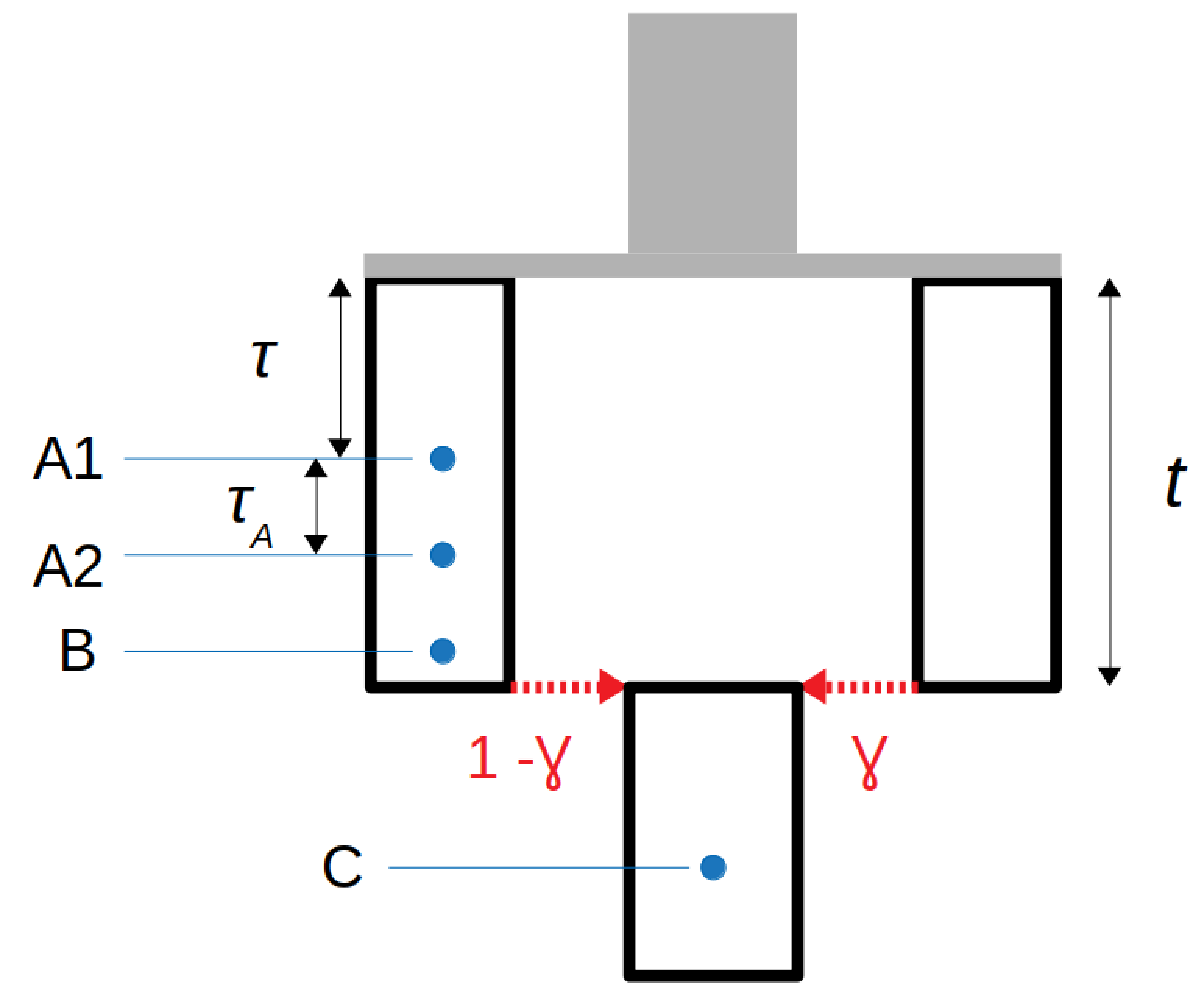
Figure 5 Simulation model set up for estimating proportion of admixture (γ) from a population diverging τ time units before anchor sample A₁.

3. Results

3.1 Simulations

3.1.1 Population continuity and ghost admixture

Figure 6 shows the mean proportion derived alleles in individuals more recent than the anchor-individual (R_d(Anchor, test)), for simulated data from models of population continuity and admixture. Forward in time, the mean proportion derived alleles remains constant under a model of population continuity even in the presence of strong branch specific genetic drift followed by population expansion (Figure 4A). Under a model of historical admixture however (Figure 4B), there are two clear successive reductions in the mean proportion derived alleles, each associated with separate admixture events. The magnitude of the reduction in proportion derived alleles decreases with the degree of drift along the branch between the anchor-individual (individual 1) and the population divergence event (t = 4, 000) with the branch leading to the population that mixes into the sampled population.

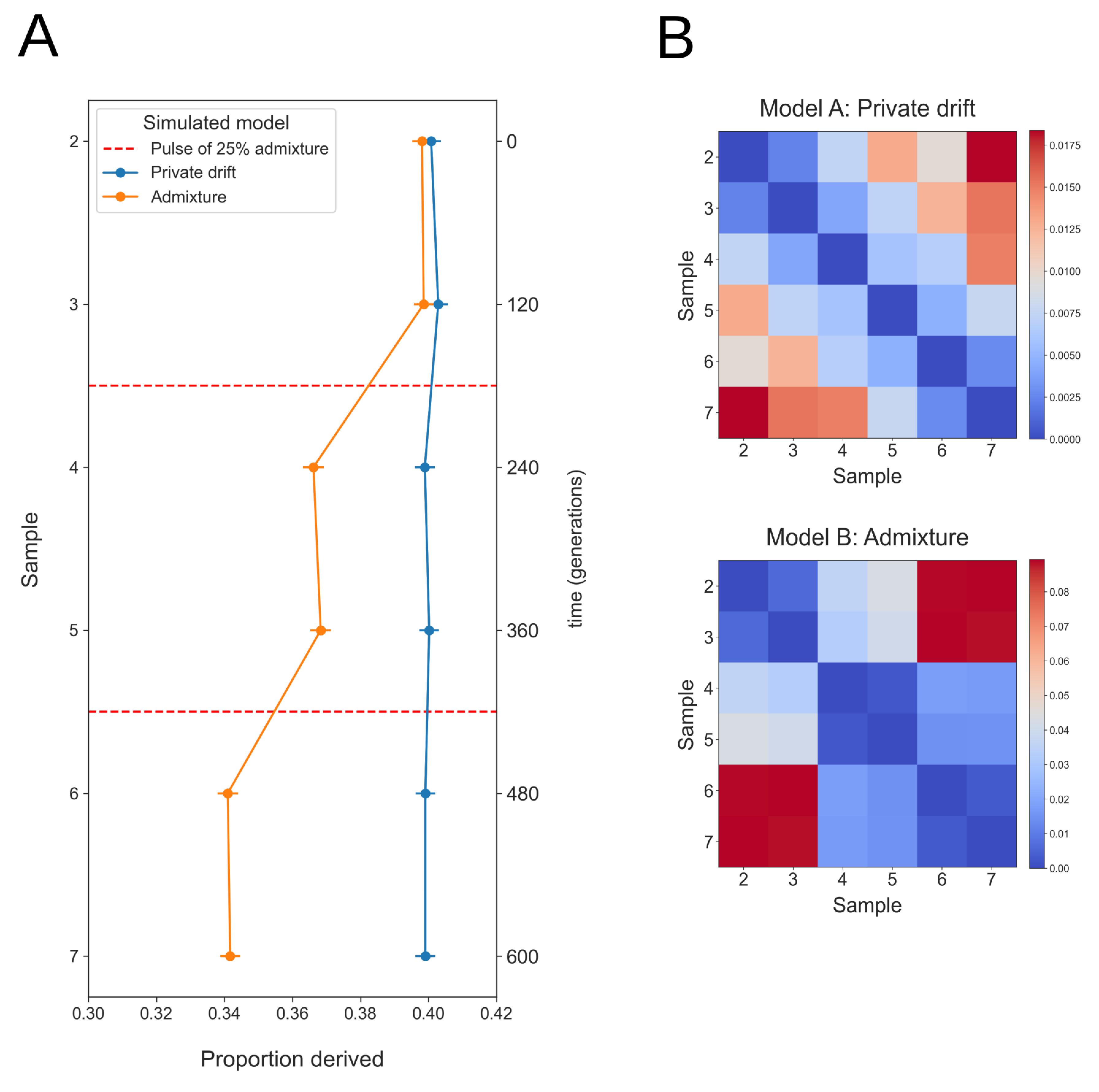
Figure 6 (A) Anchor statistic under simulated models of private drift and admixture. In each case the oldest sampled individual (1) is used as the anchor-individual, with the mean proportion derived alleles at anchor heterozygote sites counted in all more recent individuals. Red dashed lines at t = 180 & t = 420 generations indicate admixture events (25%) in the Admixture Pulse model. The mean proportion derived alleles remains constant forwards in time for individuals sampled from a model of private drift while the mean proportion derived alleles shows successive reductions for individuals sampled from a model that includes admixture. Simulated data has 1% genotyping error introduced, anchor individual coverage 8X and all more recent individuals 1X. Error bars show two weighted-block jackknife standard deviations. (B) Pairwise Fst results for the same data, showing patterns of genetic variation among samples under both models.

The simulated data used in Figure 6A has 1% sequencing error introduced for all individuals, the anchor individual down-sampled to 8X coverage and all more recent individuals (2-7) down-sampled to 1X coverage. When a genuine heterozygote site in the anchor individual is miscalled as homozygous ancestral or derived, it is excluded from the set of sites used in the analysis. When a genuine homozygous derived site is miscalled as a heterozygote in the anchor individual, and included in the set of anchor sites, there is a potential for false-positives in more recent individuals. It is for this reason that we recommend setting a threshold of 8X when calling anchor heterozygote sites. These results show that the high genotyping error rates and low coverages characteristic of ancient data do not significantly impact the power of this approach. Using a lower coverage anchor individual with an 8X threshold on heterozygote sites, will likely reduce the number of sites included in the analysis. To investigate the power of this approach with limited data, we down-sampled the number of anchor heterozygote sites used in Figure 6A to 50%, 25%, 10% and 5%. The results shown in Figure 7, demonstrate that this approach retains power to discriminate between models of population-specific drift and admixture down to 5% of anchor heterozygote sites.

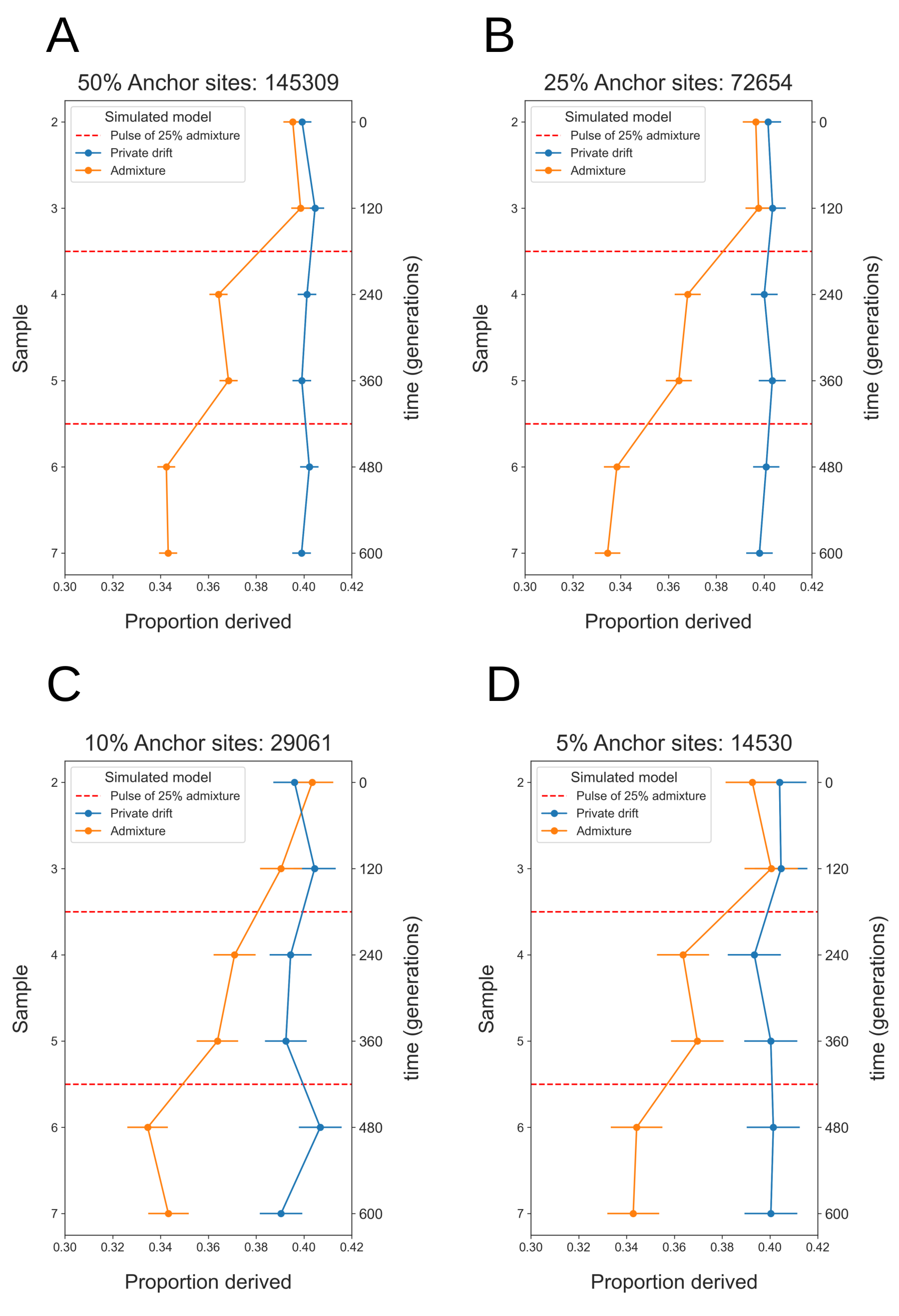
Figure 7 Anchor statistic under simulated models of private drift and admixture, with anchor heterozygote sites down-sampled to (A) 50%, (B) 25%, (C) 10% and (D) 5%. In each case the oldest sampled individual (1) is used as the anchor-individual, with the mean proportion derived alleles at anchor heterozygote sites counted in all more recent individuals. Red dashed lines at t = 180 & t = 420 generations indicate admixture events (25%) in the Admixture Pulse model. Simulated data has 1% genotyping error introduced, anchor individual coverage 8X and all more recent individuals 1X. Error bars show two weighted-block jackknife standard deviations.

3.1.2 Estimating admixture proportions

The anchor statistic can also be used to estimate admixture as outlined in the Methods section. From simulations, we show that our estimate of admixture proportion is highly correlated to the true admixture proportion (r = 0.98, Pearson correlation). Furthermore, the accuracy of the admixture-estimate does not appear to be affected by the true proportion of admixture itself (Figure 8A). Varying the population divergence time (t) from 1000 to 5500 generations does not change to accuracy of the estimation (Figure 8B). Figure 8C shows that admixture estimation uncertainty increases as the degree of drift between anchor-individuals is reduced from 0.045 to 0.005 in drift units. These observations suggest that it is not the genetic drift prior to the anchor-individuals, but rather the degree of drift between the two anchor samples that influence accuracy of admixture estimation.

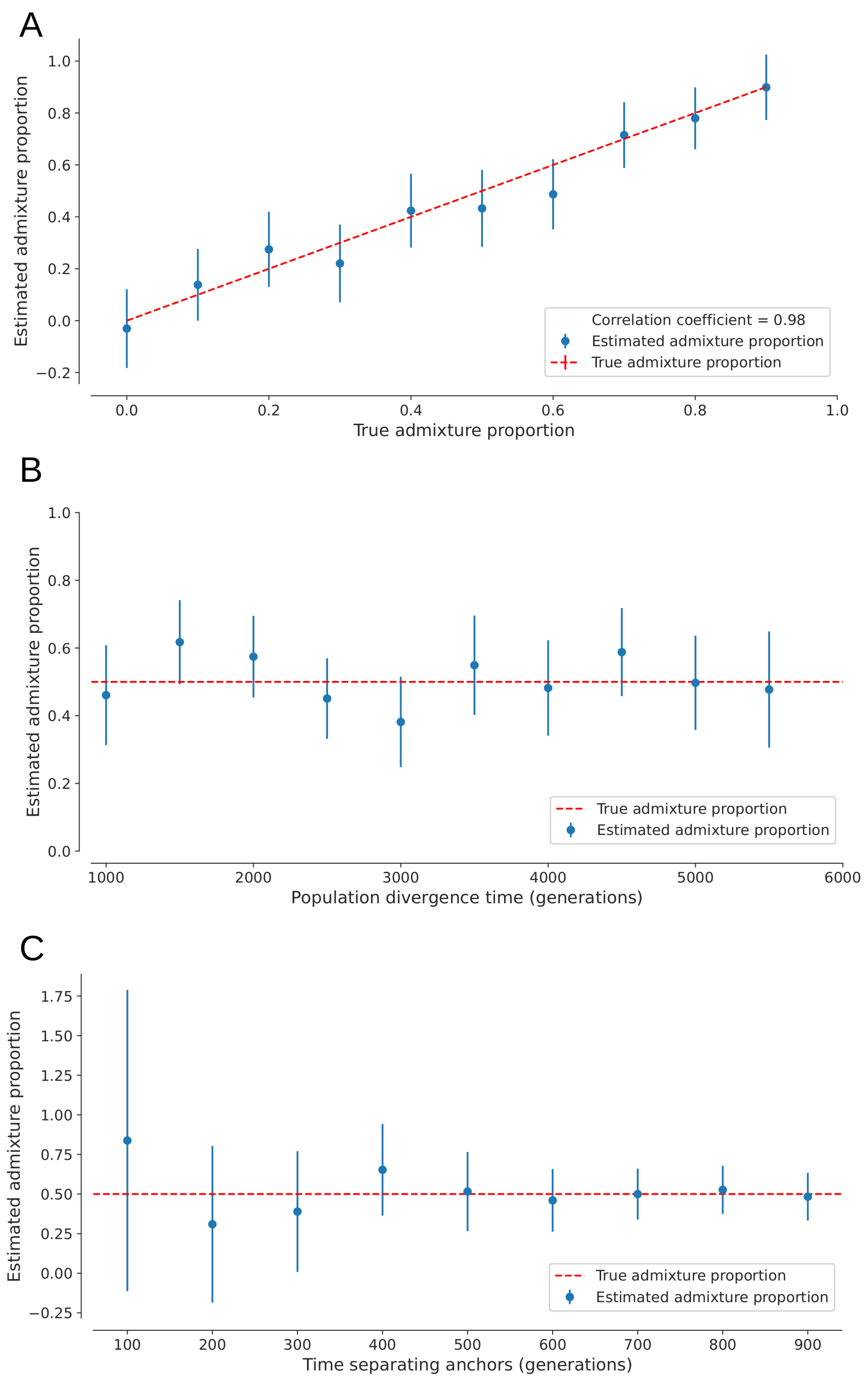
Figure 8 Estimating admixture proportions from an unsampled population with (A) a fixed divergence time (t) of 4,000 generations and admixture proportions varying from 0 to 0.9, (B) a fixed admixture proportion of 0.5 and t varying from 1,000 to 5,500 generations, and (C) a fixed admixture proportion of 0.5 and t of 4,000 generations, with time separating anchors A₁ and A₂ ranging from 100 to 900 generations. In each case, sampling time of anchor-individual A₁ is 1,000 generations and population sizes are constant at 10, 000 diploid individuals. Error bars show two weighted-block jackknife standard deviations.

Estimating admixture proportion among a temporal sample therefore requires two individuals of sufficiently high coverage that heterozygotes can be confidently called, and for those anchor individuals to be separated by enough genetic drift to gain the necessary power for accurate estimation.

3.2 Empirical data

β-drift and a convenient transformation of R_d(A,x)

Empirical data will often have a proportion erroneously called heterozygote anchor sites and it is hard to completely rule out some level of private drift associated with the anchor population. For these reasons we argue that studying –ln(R_d(A, x)) is preferable to R_d(A, x) (where A is an anchor and x is any test individual. The incentive for this is that the distance between different estimates then has a clear biological interpretation as the difference in backward drift in the path from the anchor population to the population of a test individual. For brevity, we will refer to this drift as β-drift which is always relative to some anchor population. To illustrate, consider two test individuals B and C with β-drift τ_B and τ_C relative to anchor A. If ϵ_A represents the probability of an anchor site being due to an error in the anchor sequence and not representing a a true heterozygote site and τ_A the amount of private drift associated with the anchor, then

(15)

\begin{matrix} E [R_{d} (A, B)] & = \end{matrix} (1 - ϵ_{A}) \bar{p_{A}} e^{- τ_{A}} e^{- τ_{B}}

(16)

\begin{matrix} E [R_{d} (A, C)] & = \end{matrix} (1 - ϵ_{A}) \bar{p_{A}} e^{- τ_{A}} e^{- τ_{C}}

so that

(17)

- \ln (R_{d} (A, C) + \ln (R_{d} (A, B))

is an estimate of the difference in β-drift between C and B: τ_C - τ_B.

3.2.1 Investigating population continuity from Mesolithic foragers to different Neolithic groups in Scandinavia

Scandinavia as a region holds special interest when considering the roles that population continuity and admixture have had on the emergence and spread of human cultures. It was the last region of Europe to become free of ice after the Last Glacial Maximum, and it harboured some of the last populations of hunter-gatherers in Europe. The earliest expressions of Neolithic material culture also emerged relatively late, with the arrival of the Funnelbeaker culture (FBC) circa 3500BCE to southern Scandinavia [11, 41, 42, 43]. Paleogenetic data show a close connection between these early farmers of Scandinavia and other Early and Middle Neolithic farmers of Europe [44, 45], providing strong support for a model of population discontinuity between the Scandinavian hunter-gatherers of the Mesolithic and the arriving farmers. The Neolithic Pitted Ware Culture (PWC) represents an intriguing case of a hunter-gathering culture in Scandinavia that emerge circa 3200BCE and post-dates the migration of the farmers that spread the FBC culture into Scandinavia. Despite this, the results of several studies have indicated that the PWC culture predominantly shows genetic affinity to earlier Mesolithic hunter-gatherers rather than contemporary Neolithic farmers [11, 30]. Furthermore, archaeological data has been used to paint a picture of two cultures overlapping in both time and space, coexisting in parallel for several hundred years and yet still maintaining distinct material cultures and dietary patterns, in addition to maintaining distinct genetic make-ups [2, 43, 45, 46].

We assembled a panel of fully UDG (uracil-DNA glycosylase) treated high-coverage ancient genomes from an ongoing effort to increase genome coverage from Scandinavian Stone Age humans, including a Mesolithic hunter-gatherer from the Baltic Island Stora Karlsö (sf12) and five PWC hunter-gatherers from the Baltic island of Gotland, together with five FBC farmers from the Megalithic passage tombs of Gökhem and Rössberga. In order to evaluate the impact genome coverage has on the statistics, we also included two relatively low coverage blunt-end screening genomes. One of these comes from the same ancient remains as one of the high-coverage PWC samples (ajv058) while the other one (sf9) is contemporaneous with and from the same site as sf12 (Appedix Table 2) [43,45, 46, 47]. Although from distinct material cultures, all PWC and FBC individuals are broadly contemporaneous from the same period of the Nordic Middle Neolithic (circa 3200 – 2300BCE). The raw sequence data was processed according to [48] and [47]. See Appendix section “Data processing” for how genotypes were called.

The Mesolithic hunter-gatherer sf12 was used as the anchor-individual so as to measure differences in β-drift between this individual and a set of other, more recent, individuals (Figure 9B). All PWC individuals show a similar mean β-drift that is lower compared to the FBC individuals but higher than for sf9. These results are consistent with previous findings of modest gene-flow between the contemporaneous PWC and FBC groups [2, 43, 46] but also that PWC is not a direct descendent population from SHG.

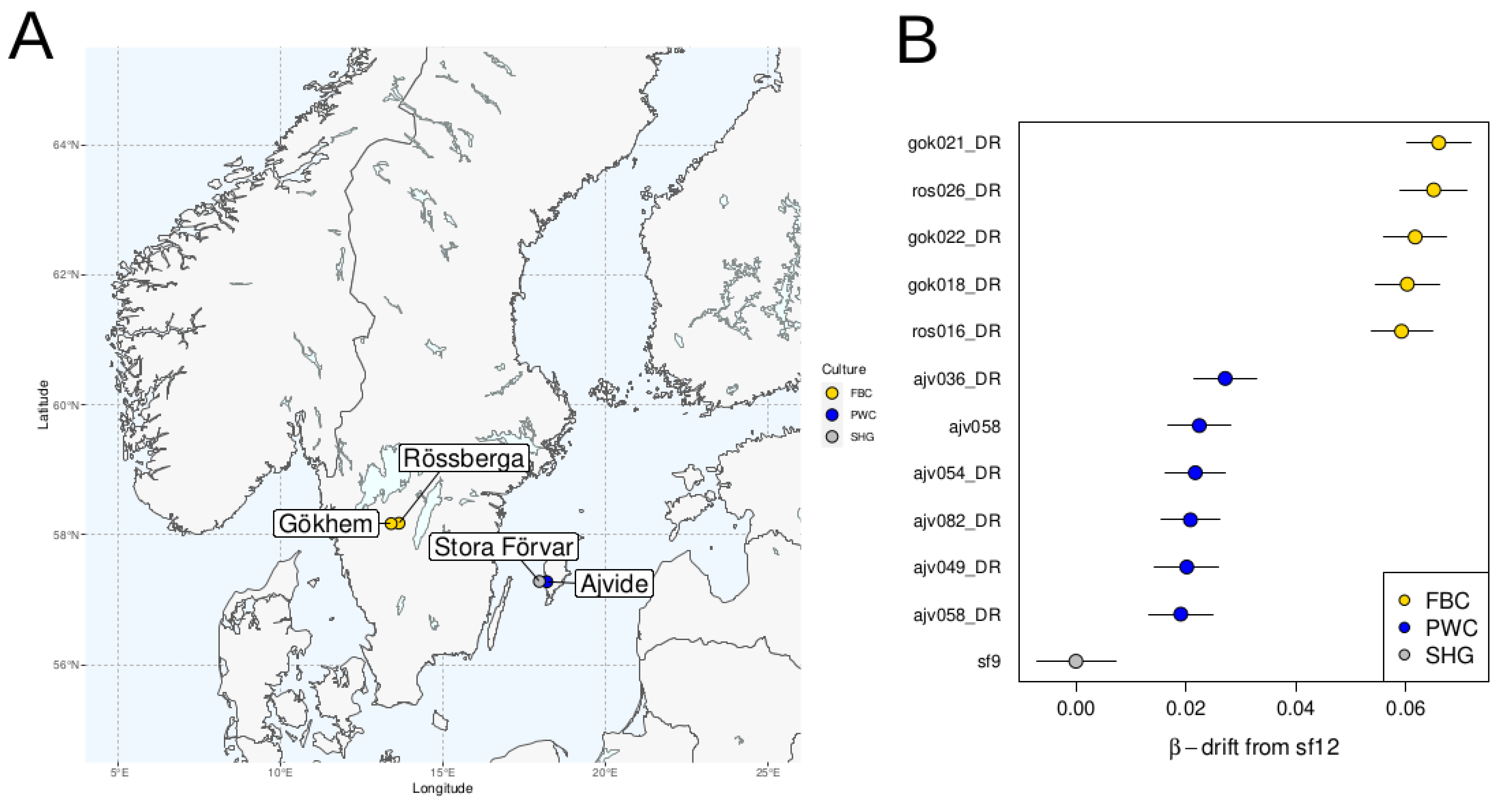
Figure 9 (A) Map showing distributions of the sampled individuals that were either representatives of the Funnel Beaker culture (FBC) or the sub-Neolithic Pitted Ware culture (PWC) during the Nordic Middle Neolithic period. All PWC individuals from Ajvide burial, Gotland. FBC burial sites sampled include Gökhem passage grave, and Rössberga passage grave. Mesolithic individuals sf9 and sf12 from Stora Förvar on Stora Karlsö. (B) β-drift relative to sf9 for different individuals with Scandinavian Mesolithic hunter-gatherer sf12 used as anchor. Error bars show two weighted-block jackknife standard deviations. The suffix “_DR” in the sample names indicate damage-repair through full UDG treatment of the sequenced libraries.

4. Discussion

Ancient genomes have the capacity to revolutionize our understanding of the demographic processes contributing to patterns of genetic variation among current-day humans as well as among other species. aDNA can reveal population continuity through time and aid in the detection of historical admixture events and population replacements. Particularly in studies of human demographic history, aDNA has proven an important resource in understanding the pre-historic movements of people that have spread cultures, languages, and technologies to new areas (e.g., [49]). In order to take full advantage of this resource however, it is essential to develop population genetic tools capable of utilizing samples of temporally distributed genomic data. Here we have outlined a novel and conceptually simple approach that is capable of elucidating questions of population continuity through time. It is sensitive to admixture from unsampled (“ghost”) populations and can take advantage of the increasing numbers of low coverage genomes available.

Although the concept of continuity is generally clear from the context (e.g., [50]), for the purpose of discussing the relationship between the anchor statistic and continuity, we will with a statement such as “an individual x has continuity level c with population A (that existed at time point t)” mean that a proportion c of all ancestors to x living at time point t belonged to population A. This in turn implies that a proportion c of x’s autosomal genetic material is expected to trace back to individuals living in population A. With respect to the different scenarios in Figure 10, this definition would imply that all test individuals in scenarios a) and b) have continuity level 1 with the anchor population while scenario c) has continuity level 0. In d), all test individuals would have some continuity level c while only the two most recent test individuals in scenario e) would have a level of continuity larger than 0.

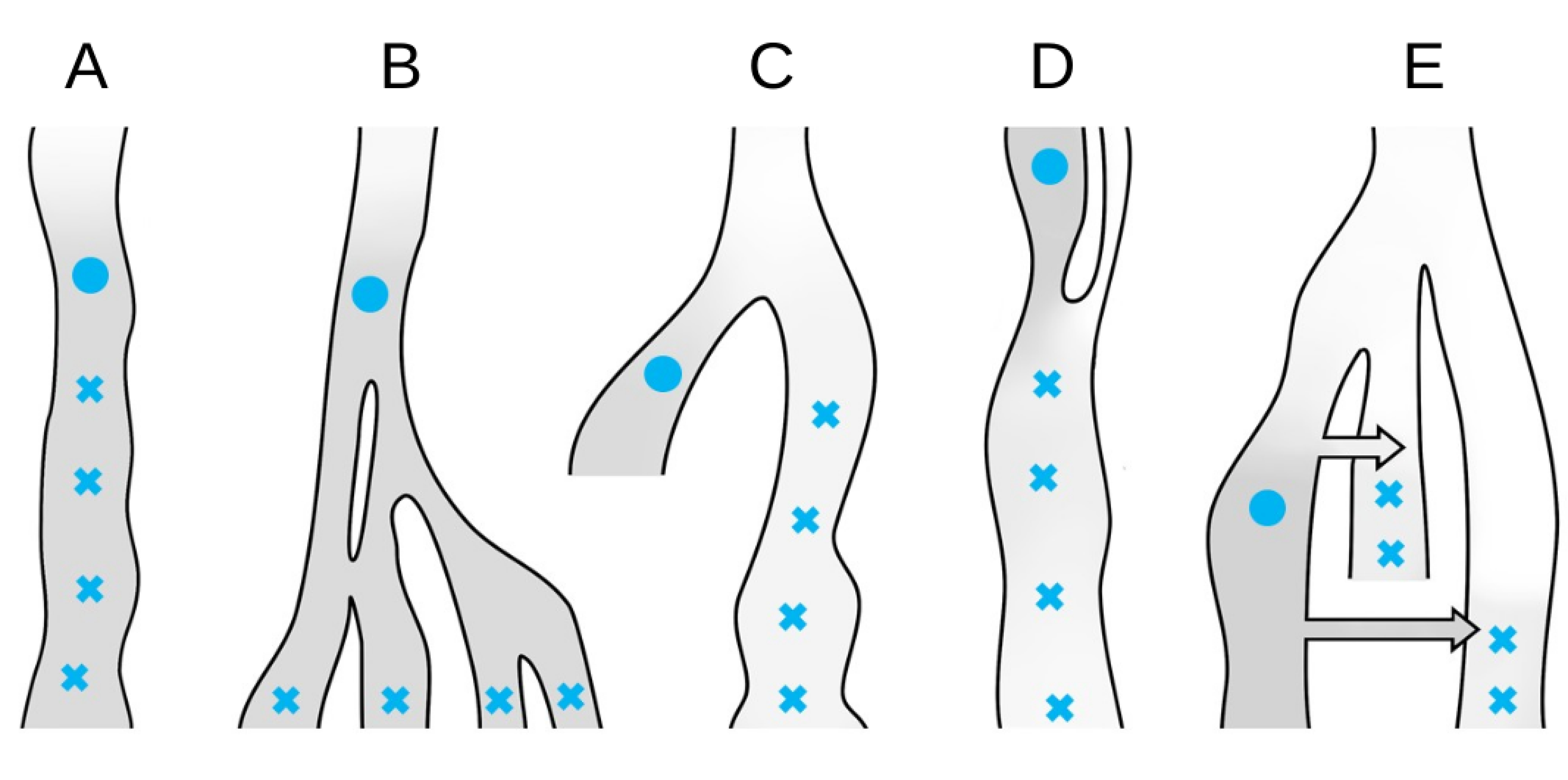
Figure 10 In each of the scenarios (A)-(D) all test individuals (blue crosses) have the same expected value of the anchor statistic when calculated relative to the anchor (blue filled circle). (e): although it will depend on the details of the two admixture events (the arrows), this scenario can result in all test individuals (blue crosses) having the same expected value of the anchor statistic. In all scenarios, the darker the grey, the lower the backward drift in the average path from the anchor population.

In contrast, all test individuals in each of the scenarios could have identical amounts of β-drift relative to the anchor. Hence, unless β-drift is 0, it can be difficult to assess any level of continuity at all based exclusively on the anchor statistic. However, when it can be assumed that one test individual has no β-drift (i.e., it has continuity level 1 with the anchor population) the absolute β-drift can be assessed. Since sf9 was sampled from the same location as sf12 and both were estimated to be around 7,000 years old (see Appendix Table 2 in the Appendix), we assumed that sf12 and sf9 were drawn from the same population and could therefore translate values of the anchor statistic to actual β-drift from the population sf12 and sf9 were sampled from.

From this analysis we conclude that although the PWC individuals have about 0.02 of β-drift relative to SHG (represented by sf12 and sf9 in this analysis) and thus that they have ancestry in other populations than SHG that were contemporaneous with SHG. Any admixture event with proportion c with a population that has an additional τ amount of β-drift such that –ln(ce^–τ + 1 – c) ≈ 0.02 would give this pattern. This is consistent with that they have none of their ancestry tracing back to SHG but to a population that diverged from SHG approximately 0.02 units of drift before the sampled individuals in this study. Alternatively, they may have a significant part of their ancestry in SHG but that they are admixed with populations that diverged considerably more than 0.02 units of drift before the population represented by sf12 and sf9. What is clear is that the FBC individuals have an additional 0.04 amount of β-drift from SHG compared to the PWC individuals.

We have shown, through simulations and an empirical example, that this approach has the power to infer population continuity and estimate proportions of ghost admixture. Although we did not find a suitable empirical example to estimate proportions of ghost admixture it is a potentially powerful aspect of our approach as the method does not require any modeling of the source of the admixture by substitute populations.

Declarations

Ethics Statement

Not applicable.

Availability of Data and Material

All software used for simulations and analysis is available at: github.com/jammc313/Genetic-continuity.

Funding

This work was funded by the Knut and Alice Wallenberg foundation and the Swedish Research Council (2022-04642)

Competing Interests

The authors have declared that no competing interests exist.

Author Contributions

Conceptualization by P.S., D.W., J.M.K. Theoretical work by P.S., D.W. Simulations and software by J.M.K. Preparation of genomic data by C.B. Analysis by J.M.K., C.B., P.S. Writing by P.S., C.B., M.J., J.M.K. Review and editing by P.S., M.J., C.B., D.W., J.M.K. Study supervised by M.J., P.S.

Acknowledgement

We want to thank Olaf Thalmann, Karl-Heinz Herzig, and Jarosoław Walkowiak for access to unpublished data, Miguel de Navascués for assistance with msprime, Nikola Vukovic for help with graphic design and Imke Lankheet for Latex assistance. This work was supported by the Knut and Alice Wallenberg foundation. The computations and data handling were enabled by resources (SNIC2022/2-11 and p2018003) provided by the Swedish National Infrastructure for Computing (SNIC) at UPPMAX.

Appendix

Moments for the population frequency

For brevity, we suppress the dependence of p and τ in the notation and write $E [X_{↓}^{n}]$ for the n’th moment of the population frequency after τ units of genetic drift forwards in time conditional on population frequency p and $E [X_{↑}^{n}]$ for the n’th moment of the population frequency going back τ units of genetic drift conditional on population frequency p. These moments are derived below.

Moments for X_↓

To derive the moments of X_↓, note that given a population frequency x of the derived variant, the probability of obtaining a sample of size n with only the derived allele is xⁿ. Thus, $X_{↓}^{n}$ is the probability to pick only the derived variant in a sample of size n, and $E [X_{↓}^{n}]$ is the expected value of this probability. Conditional on the frequency of the derived variant being p, τ time units ago, the expected probability for such a sample is derived by averaging over the number of ancestors to the sample τ time units ago, where each of those ancestors need to be of the derived type. Hence, $E [X_{↓}^{n} | X_{0} = p]$ or the expected probability to observe only the derived variant in a sample of size n is

(18)

E [X_{↓}^{n} | X_{0} = p] = \sum_{k = 1}^{n} p^{k} g_{n, k} (τ)

with g_n,k(τ) being the probability of there being k ancestors at time τ to a sample of n gene-copies (a much longer recursive proof using diffusion theory can be obtained from the authors upon request). Specifically

(19)

g_{n, k} (τ) = \frac{1}{(\binom{k}{2})} \sum_{i = k}^{n} e^{- (\binom{i}{2}) τ} (\binom{i}{2}) \prod_{l = k, l \neq i}^{n} \frac{(\binom{l}{2})}{(\binom{l}{2}) - (\binom{i}{2})}

for 2 ≤ k < n with special cases $g_{n, n} (τ) = e^{- (\binom{n}{2}) τ}$ and $g_{n, 1} (τ) = 1 - \sum_{k = 2}^{n} g_{n, k} (τ)$ [51, 52]. Since g_1,1(τ) = 1, g_2,2(τ) = e^–^τ, g_2,1 (τ) = 1 – e^–τ we have

(20)

\begin{matrix} E [X_{↓} | X_{0} = p] & = Σ_{k = 1}^{1} p^{k} g_{1, k} (τ) = p g_{1, 1} (τ) = p \end{matrix}

(21)

\begin{matrix} E [X_{↓}^{2} | X_{0} = p] & = Σ_{k = 1}^{2} p^{k} g_{2, k} (τ) = p g_{2, 1} (τ) + p^{2} g_{2, 2} (τ) \end{matrix}

(22)

= p (1 - e^{- τ}) + p^{2} e^{- τ} = p - e^{- τ} p (1 - p)

Moments for X_↑

Define ϕ(x, τ, p) to be the probability density of frequency x at time τ, given that X_A = p. The density backward in time is, in fact, the same as the forward density conditional on extinction (since by definition the derived variant goes extinct backwards in time) [53]. The forward density conditional on the allele ultimately going extinct is (using * to denote conditional on extinction)

(23)

ϕ^{*} (x, τ, p) = ϕ (x, τ, p) \frac{u_{0} (x)}{u_{0} (p)}

where u₀(z) is the probability of an allele at frequency z ultimately being lost. In a neutral model, u₀(z) = 1 – z. We get

(24)

\begin{matrix} E [X_{↑}^{n} | X_{0} = p] & = \int_{0}^{1} x^{n} ϕ^{*} (x, τ, p) d x = \int_{0}^{1} x^{n} ϕ (x, τ, p) \frac{1 - x}{1 - p} d x \end{matrix}

(25)

= \frac{1}{1 - p} (E [X_{↓}^{n} | X_{0} = p] - E [X_{↓}^{n + 1} | X_{0} = p]) .

For n = 1 we have

(26)

\begin{matrix} E [X_{↑} | X_{0} = p] & = \frac{1}{1 - p} (E [X_{↓} | X_{0} = p] - E [X_{↓}^{2} | X_{0} = p]) \end{matrix}

(27)

= \frac{1}{1 - p} (p - p + e^{- τ} p (1 - p)) = e^{- τ} p

Data processing

Before calling, a base quality score recalibration (BQSR) step was performed on the 5 terminal bases of each read by reducing the quality of all 5' T:s and all 3' A:s to phred-score 2 (#), using a custom python script. Dummy read groups (RG) were added with Picard v1.118 [57], followed by indel realignment using known indel sites in the 1000g phase1 data set [58] with GATKv. 3.5.0 [59].

A site in the anchor was chosen as an anchor position if (1) the read coverage was neither within the 5% lower or 5% upper tail of the coverage distribution (2) two variants observed at the site and the minor allele frequency was at least 1/3, (3) one of the variants could be confidently called as the ancestral variant (in our case, we demanded that all three apes had the same variant (without missingness) and that this variant was one of the variants observed in the anchor). Allele counts at anchor positions were parsed using samtools mpileup 1.17 with parameter flags -Q 30 -q 30 [60]. For site i among the anchor positions, the probability to pick the derived variant and the ancestral variant -p_d(i) and p_a(i) -for a test individual x was calculated. The anchor statistic was then calculate as

(28)

R_{d} (A, x) = \frac{Σ_{i = 1}^{L} p_{d} (i)}{Σ_{i = 1}^{L} (p_{d} (i) + p_{a} (i))}

where L is the number of anchor positions.

Simulation parameters

Table 1 Parameters used in three sets of simulations included in this study. All simulations performed in msprime, all simulation scripts available at: github.com/jammc313/Genetic-continuity/.

Sample metadata

Table 2 Information on the 10 individuals used in this study. mt, mitochondrial; cal, calibrated; BCE, before common era; PWC, Pitted Ware Culture; TRB, Funnel Beaker Culture.

References

1.	Sjödin P, Skoglund P, Jakobsson M, Blum MG, Dalen L. Assessing the Maximum Contribution from Ancient Populations. Mol Biol Evol. 2014;31(5):1248-1260. [Google Scholar] [CrossRef]

2.	Malmström H, Gilbert MT, Thomas MG, Brandström M, Storå J, Molnar P, et al. Ancient DNA reveals lack of continuity between Neolithic hunter-gatherers and contemporary Scandinavians. Curr Biol. 2009;19(20):1758-1762. [Google Scholar] [CrossRef]

3.	Green RE, Krause J, Briggs AW, Maricic T, Stenzel U, Kircher M, et al. A Draft Sequence of the Neandertal Genome. Science. 2010;328(5979):710-722. [Google Scholar] [CrossRef]

4.	Lazaridis I, Patterson N, Mittnik A, Renaud G, Mallick S, Kirsanow K, et al. Ancient human genomes suggest three ancestral populations for present-day Europeans. Nature. 2014;509(7492):409-413. [Google Scholar] [CrossRef]

5.	Raghavan M, Skoglund P, Graf KE, Metspalu M, Albrechtsen A, Moltke I, et al. The genetic prehistory of the New World Arctic. Science. 2014;345(6200):1255832. [Google Scholar] [CrossRef]

6.	Haak W, Lazaridis I, Patterson N, Rohland N, Mallick S, Llamas B, et al. Massive migration from the steppe was a source for Indo-European languages in Europe. Nature. 2015;522(7555):207-211. [Google Scholar] [CrossRef]

7.	Rasmussen M, Anzick SL, Waters MR, Skoglund P, DeGiorgio M, Stafford TW Jr, et al. The ancestry and affiliations of Kennewick Man. Nature. 2015;523(7561):455-458. [Google Scholar] [CrossRef]

8.	Lazaridis I, Nadel D, Rollefson G, Merrett DC, Rohland N, Mallick S, et al. Genomic insights into the origin of farming in the ancient Near East. Nature. 2016;536(7617):419-424. [Google Scholar] [CrossRef]

9.	Slatkin M. Statistical methods for analyzing ancient DNA from hominins. Curr Opin Genet Dev. 2016;41:72-76. [Google Scholar] [CrossRef]

10.	Schraiber JG. Assessing the Relationship of Ancient and Modern Populations. Genetics. 2017;205(2):833-852. [Google Scholar] [CrossRef]

11.	Skoglund P, Malmström H, Omrak A, Raghavan M, Valdiosera C, Günther T, et al. Origins and genetic legacy of Neolithic farmers and hunter-gatherers in Europe. Science. 2012;336(6080):466-469. [Google Scholar] [CrossRef]

12.	Olalde I, Brace S, Allentoft ME, Armit I, Kristiansen K, Booth T, et al. The Beaker phenomenon and the genomic transformation of northwest Europe. Nature. 2018;555(7695):190-196. [Google Scholar] [CrossRef]

13.	Beerli P. Effect of unsampled populations on the estimation of population sizes and migration rates between sampled populations. Mol Ecol. 2004;13:827-836. [Google Scholar] [CrossRef]

14.	Slatkin M. Seeing ghosts: the effect of unsampled populations on migration rates estimated for sampled populations. Mol Ecol. 2005;14:67-73. [Google Scholar] [CrossRef]

15.	Lawson DJ, van Dorp L, Falush D. A tutorial on how not to over-interpret STRUCTURE and ADMIXTURE bar plots. Nat Commun. 2018;9:3258. [Google Scholar] [CrossRef]

16.	Städler T, Haubold B, Merino C, Stephan W, Pfaffelhuber P. The impact of sampling schemes on the site frequency spectrum in nonequilibrium subdivided populations. Genetics. 2009;182(1):205-216. [Google Scholar] [CrossRef]

17.	Rosen Z, Schaffner SF, Pe’er I, Sabeti PC. Geometry of the Sample Frequency Spectrum and the Perils of Demographic Inference. Genetics. 2018;210(2):665-682. [Google Scholar] [CrossRef]

18.	Mazet O, Rodríguez W, Chikhi L. Demographic inference using structure-aware approaches. Heredity. 2016;116:362-371. [Google Scholar] [CrossRef]

19.	McVean G. A genealogical interpretation of principal components analysis. PLoS Genet. 2009;5(10):e1000686. [Google Scholar] [CrossRef]

20.	François O, Blum MG, Jakobsson M, Rosenberg NA. Inference of population genetic structure from temporal samples of DNA. bioRxiv. 2019. [Google Scholar] [CrossRef]

21.	Reich D, Green RE, Kircher M, Krause J, Patterson N, Durand EY, et al. Genetic history of an archaic hominin group from Denisova Cave in Siberia. Nature. 2010;468(7327):1053-1060. [Google Scholar] [CrossRef]

22.	Wall JD, Yang MA, Jay F, Kim SY, Durand EY, Stevison LS, et al. Identification of African-specific admixture between modern and archaic humans. Am J Hum Genet. 2019;105(6):1254-1261. [Google Scholar] [CrossRef]

23.	Durvasula A, Sankararaman S. Recovering signals of ghost archaic introgression in African populations. Sci Adv. 2020;6(7). [Google Scholar] [CrossRef]

24.	Skov L, Peyrégne S, Meier JI, Welch R, Racimo F, Kelso J, et al. Detecting archaic introgression using an unadmixed outgroup. PLoS Genet. 2018;14(9):1-15. [Google Scholar] [CrossRef]

25.	Allentoft ME, Collins M, Harker D, Haile J, Oskam CL, Hale ML, et al. The half-life of DNA in bone: measuring decay kinetics in 158 dated fossils. Proc Biol Sci. 2012;279(1748):4724-4733. [Google Scholar] [CrossRef]

26.	Skoglund P, Jakobsson M, Götherström A, Stora J. Separating endogenous ancient DNA from modern day contamination in a Siberian Neandertal. Proc Natl Acad Sci U S A. 2014;111(6):2229-2234. [Google Scholar] [CrossRef]

27.	Dabney J, Meyer M, Shapiro B, Hofreiter M. Extraction ofhighly degraded DNA from ancient bones and teeth. Ancient DNA. New York, USA: Springer; 2019. p.25-29. [Google Scholar] [CrossRef]

28.	Wang C, Zollner S, Rosenberg NA. A quantitative comparison of the similarity between genes and geography in worldwide human populations. PLoS Genet. 2012;8(8):e1002886. [Google Scholar] [CrossRef]

29.	Verdu P, Becker NS, Froment A, Georges M, Grugni V, Quintana-Murci L, et al. Patterns of Admixture and Population Structure in Native Populations of Northwest North America. PLoS Genet. 2014;10(8):e1004530. [Google Scholar] [CrossRef]

30.	Skoglund P, Sjödin P, Skoglund T, Lascoux M, Jakobsson M. Investigating Population History Using Temporal Genetic Differentiation. Mol Biol Evol. 2014;31(9):2516-2527. [Google Scholar] [CrossRef]

31.	Diego-Ortega-Del V, Montgomery S. FST between Archaic and Present-Day Samples. Heredity. 2019;122:711-718. [Google Scholar] [CrossRef]

32.	Patterson N, Moorjani P, Luo Y, Mallick S, Rohland N, Zhan Y, et al. Ancient admixture in human history. Genetics. 2012;192(3):1065-1093. [Google Scholar] [CrossRef]

33.	Yang MA, Montgomery S. Using Ancient Samples in Projection Analysis. G3 (Bethesda). 2015;6(1):99-105. [Google Scholar] [CrossRef]

34.	Racimo F, Renaud G, Slatkin M. Joint Estimation of Contamination, Error and Demography for Nuclear DNA from Ancient Humans. PLoS Genet. 2016;12(4):e1005972. [Google Scholar] [CrossRef]

35.	Silva NM, Jorde LB, Ferreira AM, Rocha J. Bayesian estimation of partial population continuity using ancient DNA and spatially explicit simulations. Evol Appl. 2018;11(9):1642-1655. [Google Scholar] [CrossRef]

36.	François O, Jay F. Factor analysis of ancient population genomic samples. Nat Commun. 2020;11(1):4661. [Google Scholar] [CrossRef]

37.	Novembre J, Stephens M. Interpreting principal component analyses of spatial population genetic variation. Nat Genet. 2008;40:646-649. [Google Scholar] [CrossRef]

38.	Kimura M, Ohta T. The average number of generations until fixation of a mutant gene in a population. Genetics. 1969;61(3):763-771. [Google Scholar] [CrossRef]

39.	Kelleher J, Etheridge AM, McVean G. Efficient Coalescent Simulation and Genealogical Analysis for Large Sample Sizes. PLoS Comput Biol. 2016;12(5):e1004842. [Google Scholar] [CrossRef]

40.	Miles A, Kelleher J, Millar T, Pisupati R, Rae S, Ralph P, et al. cggh/scikit-allel: v1.3.8. (Version v1.3.8.) Zenodo. 2024.

41.	Midgley M. TRB culture: The first farmers of the north European plain. Edinburgh, UK: Edinburgh University Press; 1992. [Google Scholar]

42.	Price DT, editor. Europe’s first farmers. Cambridge, UK: Cambridge University Press; 2000. [Google Scholar] [CrossRef]

43.	Fraser M, Sjögren KG, Knipper C, Philippsen B, Lidén K. New insights on cultural dualism and population structure in the Middle Neolithic Funnel Beaker culture on the island of Gotland. J Archaeol Sci Rep. 2018;17:325-334. [Google Scholar] [CrossRef]

44.

Malmström H, Linderholm A, Skoglund P, Storå J, Sjödin P, Gilbert MTP, et al. Ancient mitochondrial DNA from the northern fringe of the Neolithic farming expansion in Europe sheds light on the dispersion process. Philos Trans R Soc Lond B Biol Sci. 2015;370(1660):20130373. [Google Scholar] [CrossRef]

45.	Malmström H, Linderholm A, Skoglund P, Storå J, Sjögren KG, Gilbert MT, et al. The genomic ancestry of the Scandinavian Battle Axe Culture people and their relation to the broader Corded Ware horizon. Proc Biol Sci. 2019;286(1905):20191528. [Google Scholar] [CrossRef]

46.	Coutinho A, Dørum Å, Almstetter L, Sjögren KG, Krzewińska M, Larsson M, et al. The Neolithic Pitted Ware culture foragers were culturally but not genetically influenced by the Battle Axe culture herders. Am J Phys Anthropol. 2020;172(4):638-649. [Google Scholar] [CrossRef]

47.	Günther T, Malmström H, Svensson EM, Omrak A, Sánchez-Quinto FA, Kılınç GM, et al. Population genomics of Mesolithic Scandinavia: Investigating early postglacial migration routes and high-latitude adaptation. PLoS Biol. 2018;16(1):e2003703. [Google Scholar] [CrossRef]

48.	Alves I, Houet R, Larmuseau MH, Maisongrande A, Sidore C, Zoledziewska M, et al. Genetic population structure across Brittany and the downstream Loire basin provides new insights on the demographic history of Western Europe. bioRxiv. 2022. [Google Scholar] [CrossRef]

49.	Arcos MC, Ávila MC, Schlebusch CR. Going local with ancient DNA: A review of human histories from regional perspectives. Science. 2023;382(6666):53-58. [Google Scholar] [CrossRef]

50.	Mattila TM, Svensson EM, Juras A, Günther T, Kashuba N, Ala-Hulkko T, et al. Genetic continuity, isolation, and gene flow in Stone Age Central and Eastern Europe. Commun Biol. 2023;6:793. [Google Scholar] [CrossRef]

51.	Tavaré S. Line-of-Descent and Genealogical Processes, and Their Applications in Population Genetics Models. Theor Popul Biol. 1984;26(1):119-164. [Google Scholar] [CrossRef]

52.	Wakeley J. Coalescent Theory: An Introduction. 1st ed.. Greenwood Village, Colorado, USA: Roberts Company Publishers; 2009. [Google Scholar]

53.	Griffiths RC. The frequency spectrum of a mutation, and its age, in a general diffusion model. Theor Popul Biol. 2003;64:241-251. [Google Scholar] [CrossRef]

54.	Wallin P, Martinsson-Wallin H. Decoding Neolithic Atlantic and Mediterranean Island Ritual. Collective spaces and material expressions: ritual practice and island identities in Neolithic Gotland. Oxford, UK: Oxbow Books; 2016. In:. [Google Scholar]

55.	Paulsson BS. Scandinavian models: Radiocarbon dates and the origin and spreading of passage graves in Sweden and Denmark. Radiocarbon. 2010;52(3):1002-1017. [Google Scholar]

56.	Blank M, Sjögren KG, Storå J. Old bones or early graves? Megalithic burial sequences in southern Sweden based on 14C datings. Archaeol Anthropol Sci. 2020;12:89. [Google Scholar] [CrossRef]

57.	Picard Toolkit. Broad Institute. [cited 2022 Jul 10]. Available from: https://broadinstitute.github.io/picard.

58.	1000 Genomes Project Consortium. An integrated map of genetic variation from 1,092 human genomes. Nature. 2012;491:56-65. [Google Scholar] [CrossRef]

59.	Van der Auwera G, O’Connor BD. Genomics in the Cloud: Using Docker, GATK, and WDL in Terra. O’Reilly Media, Incorporated; 2020.

60.	Li H. A statistical framework for SNP calling, mutation discovery, association mapping and population genetical parameter estimation from sequencing data. Bioinformatics. 2011;27(21):2987-2993. [Google Scholar] [CrossRef]

Download PDF

Share this article

Parameters common to all sets of simulations
Number of runs	1000
Length of sequence	2 Mb
Recombination rate	1.25e-8
Mutation rate	1.45e-8
Generation time (years)	29
Simulation set 1: Confounding effects of temporal structure
Parameter	Demographic Model A	Demographic Model B
Pop1-Pop2 divergence time (yrs)	55000	55000
Pop2-Pop3 divergence time (yrs)	-	200000
Ancestral Pop size	1000	1000
Pop1 size	1000	1000
Initial Pop2 size	1000	1000
End Pop2 size	100	1000
Admixture pulse time (yrs)	-	35000
Admixture pulse	-	30%
Anchor sample time	50000	50000
Admixing Pop size	-	5000
Simulation set 2: Discriminating population continuity from admixture
Parameter	Demographic Model A	Demographic Model B
Pop1-Pop2 divergence time (gens)	4000	4000
Ancestral Pop size	10000	10000
Initial Pop1 size	10000	1000
End Pop1 size	1000	1000
Pop2 size	10000	10000
Admixture pulse 1 time (yrs)	-	420
Admixture pulse 1 time (yrs)	-	120
Admixture pulses	-	25%
Sequencing error	1%	1%
Sampling times (gens)	1: 720, 2: 600, 3: 480, 4: 360, 5: 240, 6: 120, 7: 0
Sample coverages	1: 8X, 2: 1X, 3: 1X, 4: 1X, 5: 240, 6: 1X, 7: 1X
Simulation set 3: Estimating admixture proportions
Ancestral Pop size	10000	10000
Pop1 size	10000	10000
Pop2 size	10000	10000
Admixture pulse time (gens)	25	25
Admixture proportion	0-0.9
Pop1-Pop2 divergence time (gens)	1000-6000
Time separating anchors (gens)	100-900

Sample	Context	Origin	Genome coverage	Contamination (%)		Source	Age (cal. years BCE)	Genetic sex
Sample	Context	Origin	Genome coverage	mt	autosomal	Source	Age (cal. years BCE)	Genetic sex
sf12	Mesolithic	Stora Förvar,per Stora Karlsö	62.16	0.015	0.73	[47]	7083-6807	XX
sf9	Mesolithic	Stora Förvar, Stora Karlsö	1.15	5.36	0	[47]	7350-7038	XX
ajv36	PWC	Ajvide, Gotland	10.96	0.029	0.69	[46]	3200-2300	XX
ajv49	PWC	Ajvide, Gotland	20.26	0.049	0.66	Unpublished	3200-2300	XY
ajv54	PWC	Ajvide, Gotland	17.83	0.024	0.47	[45]	3200-2300	XY
ajv58	PWC	Ajvide, Gotland	17.21	0.045	0.53	[30]	2950-2650	XY
ajv82	PWC	Ajvide, Gotland	20.88	0.185	0.65	[54]	3200-2300	XY
gok18	TRB	Gökhem, Västergötland	14.64	0.089	0.75	[55]	3760-3340	XY
gok21	TRB	Gökhem, Västergötland	13.14	0.158	1.11	[55]	3760-3340	XY
gok22	TRB	Gökhem, Västergötland	13.90	0.205	1.07	[55]	3760-3340	XY
ros16	TRB	Rössberga, Västergötland	19.53	0.065	0.62	[56]	3082-2894	XX